Confidence intervals and profile likelihoods for parameters in cumulative link models

Computes confidence intervals from the profiled likelihood for one or more parameters in a fitted cumulative link model, or plots the profile likelihood function.

Usage

# S3 method for class 'clm2'
confint(object, parm, level = 0.95, whichL = seq_len(p),
        whichS = seq_len(k), lambda = TRUE, trace = 0, ...)

# S3 method for class 'profile.clm2'
confint(object, parm = seq_along(Pnames), level = 0.95, ...)

# S3 method for class 'clm2'
profile(fitted, whichL = seq_len(p), whichS = seq_len(k),
        lambda = TRUE, alpha = 0.01, maxSteps = 50, delta = LrootMax/10,
        trace = 0, stepWarn = 8, ...)

# S3 method for class 'profile.clm2'
plot(x, parm = seq_along(Pnames), level = c(0.95, 0.99),
        Log = FALSE, relative = TRUE, fig = TRUE, n = 1e3, ..., ylim = NULL)

Arguments

object

a fitted clm2 object or a profile.clm2 object.

fitted

a fitted clm2 object.

x

a profile.clm2 object.

parm

not used in confint.clm2.

For confint.profile.clm2: a specification of which parameters are to be given confidence intervals, either a vector of numbers or a vector of names. If missing, all parameters are considered.

For plot.profile.clm2: a specification of which parameters the profile likelihood are to be plotted for, either a vector of numbers or a vector of names. If missing, all parameters are considered.

level

the confidence level required.

whichL

a specification of which location parameters are to be given confidence intervals, either a vector of numbers or a vector of names. If missing, all location parameters are considered.

whichS

a specification of which scale parameters are to be given confidence intervals, either a vector of numbers or a vector of names. If missing, all scale parameters are considered.

lambda

logical. Should profile or confidence intervals be computed for the link function parameter? Only used when one of the flexible link functions are used; see the link-argument in clm2.

trace

logical. Should profiling be traced?

alpha

Determines the range of profiling. By default the likelihood is profiled in the 99% confidence interval region as determined by the profile likelihood.

maxSteps

the maximum number of profiling steps in each direction (up and down) for each parameter.

delta

the length of profiling steps. To some extent this parameter determines the degree of accuracy of the profile likelihood in that smaller values, i.e. smaller steps gives a higher accuracy. Note however that a spline interpolation is used when constructing confidence intervals so fairly long steps can provide high accuracy.

stepWarn

a warning is issued if the no. steps in each direction (up or down) for a parameter is less than stepWarn (defaults to 8 steps) because this indicates an unreliable profile.

Log

should the profile likelihood be plotted on the log-scale?

relative

should the relative or the absolute likelihood be plotted?

fig

should the profile likelihood be plotted?

n

the no. points used in the spline interpolation of the profile likelihood.

ylim

overrules default y-limits on the plot of the profile likelihood.

...

additional argument(s) for methods including range (for the hidden function profileLambda) that sets the range of values of lambda at which the likelihood should be profiled for this parameter.

Value

confint: A matrix (or vector) with columns giving lower and upper confidence limits for each parameter. These will be labelled as (1-level)/2 and 1 - (1-level)/2 in % (by default 2.5% and 97.5%). The parameter names are preceded with "loc." or "sca." to indicate whether the confidence interval applies to a location or a scale parameter.

plot.profile.clm2 invisibly returns the profile object.

Details

These confint methods call the appropriate profile method, then finds the confidence intervals by interpolation of the profile traces. If the profile object is already available, this should be used as the main argument rather than the fitted model object itself.

In plot.profile.clm2: at least one of Log and relative arguments have to be TRUE.

Author

Rune Haubo B Christensen

See also

profile and confint

Examples

options(contrasts = c("contr.treatment", "contr.poly"))

## More manageable data set:
(tab26 <- with(soup, table("Product" = PROD, "Response" = SURENESS)))
#>        Response
#> Product   1   2   3   4   5   6
#>    Ref  132 161  65  41 121 219
#>    Test  96  99  50  57 156 650
dimnames(tab26)[[2]] <- c("Sure", "Not Sure", "Guess", "Guess", "Not Sure", "Sure")
dat26 <- expand.grid(sureness = as.factor(1:6), prod = c("Ref", "Test"))
dat26$wghts <- c(t(tab26))

m1 <- clm2(sureness ~ prod, scale = ~prod, data = dat26,
          weights = wghts, link = "logistic")

## profile
pr1 <- profile(m1)
#> Error in eval(expr, p): object 'dat26' not found
par(mfrow = c(2, 2))
plot(pr1)
#> Error: object 'pr1' not found

m9 <- update(m1, link = "log-gamma")
pr9 <- profile(m9, whichL = numeric(0), whichS = numeric(0))
#> Error in eval(expr, p): object 'dat26' not found
par(mfrow = c(1, 1))
plot(pr9)
#> Error: object 'pr9' not found

plot(pr9, Log=TRUE, relative = TRUE)
#> Error: object 'pr9' not found
plot(pr9, Log=TRUE, relative = TRUE, ylim = c(-4, 0))
#> Error: object 'pr9' not found
plot(pr9, Log=TRUE, relative = FALSE)
#> Error: object 'pr9' not found

## confint
confint(pr9)
#> Error: object 'pr9' not found
confint(pr1)
#> Error: object 'pr1' not found

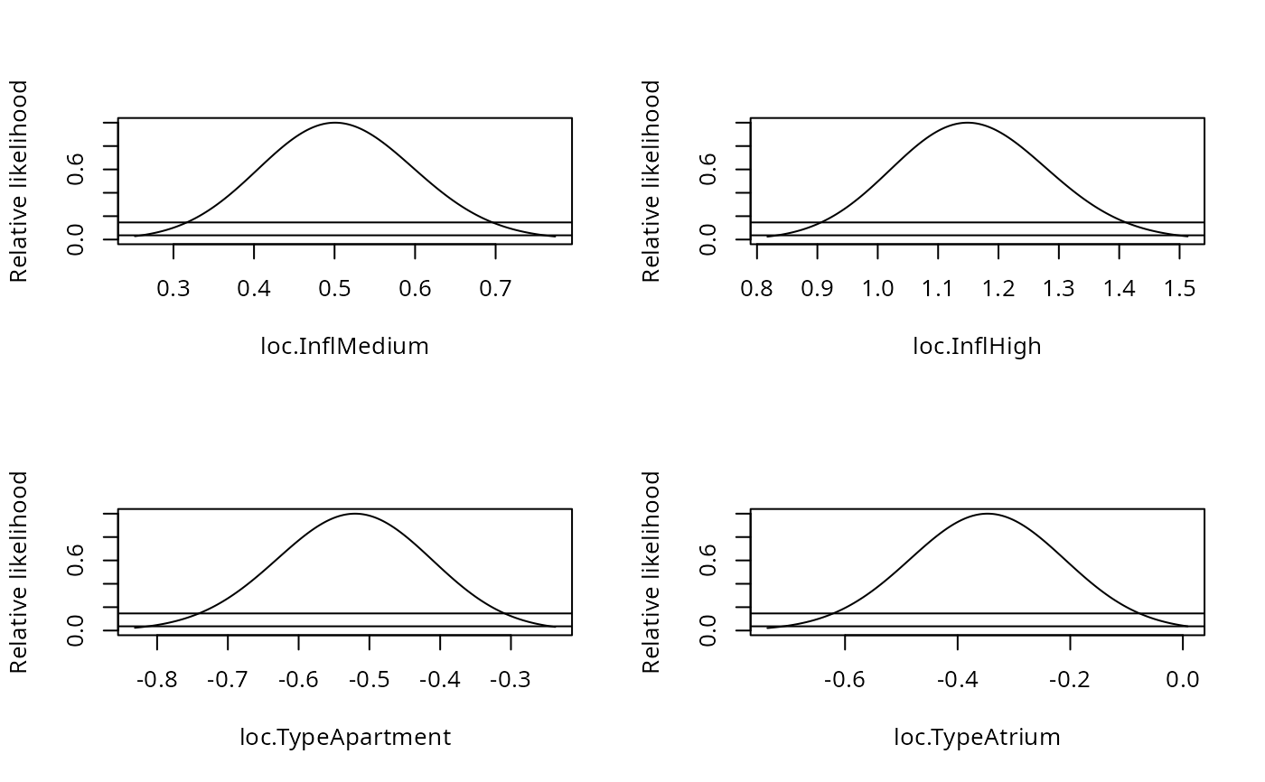
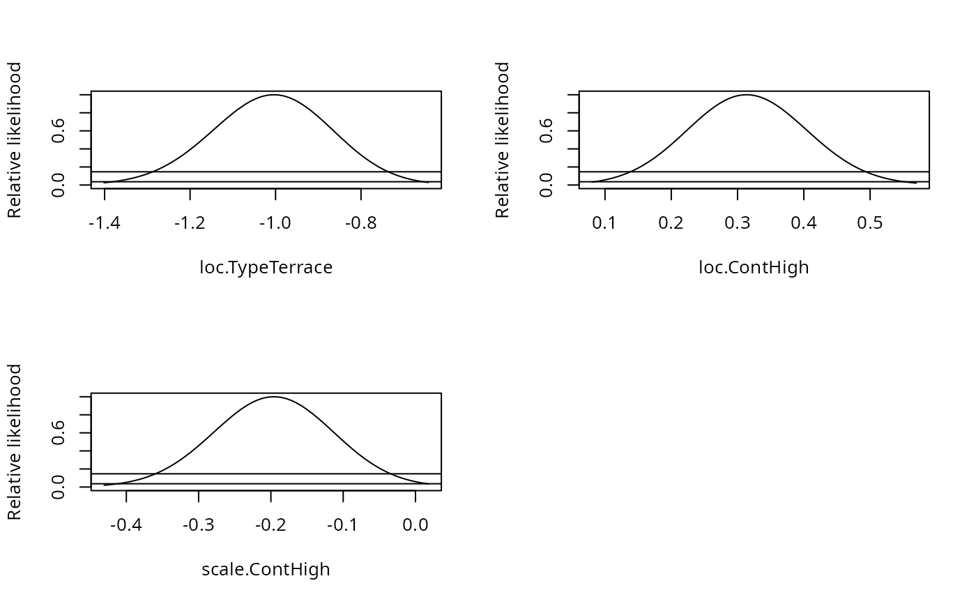
## Extend example from polr in package MASS:
## Fit model from polr example:
if(require(MASS)) {
    fm1 <- clm2(Sat ~ Infl + Type + Cont, scale = ~ Cont, weights = Freq,
                data = housing)
    pr1 <- profile(fm1)
    confint(pr1)
    par(mfrow=c(2,2))
    plot(pr1)
}