Multivariate Normal Density and Random Deviates
Mvnorm.RdThese functions provide the density function and a random number
generator for the multivariate normal
distribution with mean equal to mean and covariance matrix
sigma.
Arguments
- x
vector or matrix of quantiles. When
xis a matrix, each row is taken to be a quantile and columns correspond to the number of dimensions,p.- n
number of observations.
- mean
mean vector, default is
rep(0, length = ncol(x)). Inldmvnormorsldmvnorm,meanis a matrix with observation-specific means arranged in columns.- sigma
covariance matrix, default is
diag(ncol(x)).- log
logical; if
TRUE, densities d are given as log(d).- method
string specifying the matrix decomposition used to determine the matrix root of
sigma. Possible methods are eigenvalue decomposition ("eigen", default), singular value decomposition ("svd"), and Cholesky decomposition ("chol"). The Cholesky is typically fastest, not by much though.- pre0.9_9994
logical; if
FALSE, the output produced in mvtnorm versions up to 0.9-9993 is reproduced. In 0.9-9994, the output is organized such thatrmvnorm(10,...)has the same first ten rows asrmvnorm(100, ...)when called with the same seed.- checkSymmetry
logical; if
FALSE, skip checking whether the covariance matrix is symmetric or not. This will speed up the computation but may cause unexpected outputs when ill-behavedsigmais provided. The default value isTRUE.- rnorm
a function with the same interface as
rnorm. This allows switching to other generators of standard normal variables.
Details
dmvnorm computes the density function of the multivariate normal
specified by mean and the covariance matrix sigma.
rmvnorm generates multivariate normal variables.
Examples
dmvnorm(x=c(0,0))
#> [1] 0.1591549
dmvnorm(x=c(0,0), mean=c(1,1))
#> [1] 0.05854983

sigma <- matrix(c(4,2,2,3), ncol=2)
x <- rmvnorm(n=500, mean=c(1,2), sigma=sigma)
colMeans(x)
#> [1] 1.017563 2.004162
var(x)
#>          [,1]     [,2]
#> [1,] 4.052903 2.044061
#> [2,] 2.044061 3.008296
dS <- dmvnorm(x, sigma = sigma)

### alternative interface
C <- t(chol(sigma))
(C <- ltMatrices(C[lower.tri(C, diag = TRUE)], diag = TRUE))
#> , , 1
#>
#>          1        2
#> 1 2.000000        .
#> 2 1.000000 1.414214
#>
dC <- exp(ldmvnorm(obs = t(x), chol = C, logLik = FALSE))
all.equal(dS, dC)
#> [1] TRUE

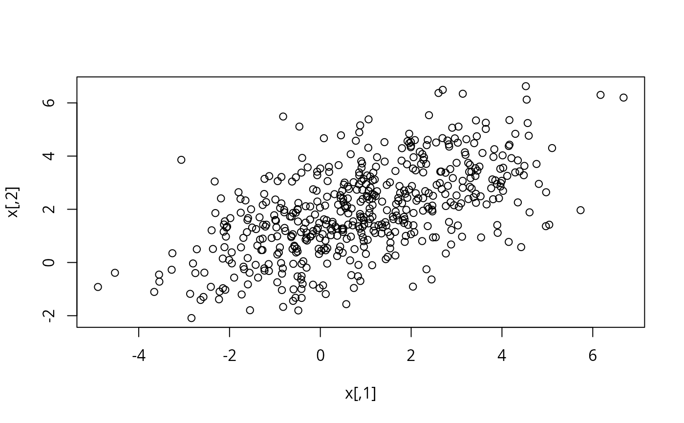
x <- rmvnorm(n=500, mean=c(1,2), sigma=sigma, method="chol")
colMeans(x)
#> [1] 0.9191267 1.9707497
var(x)
#>          [,1]     [,2]
#> [1,] 3.813205 1.900035
#> [2,] 1.900035 2.784946

plot(x)