Methods for General Linear Hypotheses — glht-methods • multcomp

Simultaneous tests and confidence intervals for general linear hypotheses.

Usage

# S3 method for class 'glht'
summary(object, test = adjusted(), ...)
# S3 method for class 'glht'
confint(object, parm, level = 0.95, calpha = adjusted_calpha(), 
        ...)
# S3 method for class 'glht'
coef(object, rhs = FALSE, ...)
# S3 method for class 'glht'
vcov(object, ...)
# S3 method for class 'confint.glht'
plot(x, xlim, xlab, ylim, ...)
# S3 method for class 'glht'
plot(x, ...)
univariate()
adjusted(type = c("single-step", "Shaffer", "Westfall", "free", 
         p.adjust.methods), ...)
Ftest()
Chisqtest()
adjusted_calpha(...)
univariate_calpha(...)

Arguments

object: an object of class glht.
test: a function for computing p values.
parm: additional parameters, currently ignored.
level: the confidence level required.
calpha: either a function computing the critical value or the critical value itself.
rhs: logical, indicating whether the linear function \(K \hat{\theta}\) or the right hand side \(m\) (rhs = TRUE) of the linear hypothesis should be returned.
type: the multiplicity adjustment (adjusted) to be applied. See below and p.adjust.
x: an object of class glht or confint.glht.
xlim: the x limits (x1, x2) of the plot.
ylim: the y limits of the plot.
xlab: a label for the x axis.
...: additional arguments, such as maxpts, abseps or releps to pmvnorm in adjusted or qmvnorm in confint. Note that additional arguments specified to summary, confint, coef and vcov methods are currently ignored.

Details

The methods for general linear hypotheses as described by objects returned by glht can be used to actually test the global null hypothesis, each of the partial hypotheses and for simultaneous confidence intervals for the linear function \(K \theta\).

The coef and vcov methods compute the linear function \(K \hat{\theta}\) and its covariance, respectively.

The test argument to summary takes a function specifying the type of test to be applied. Classical Chisq (Wald test) or F statistics for testing the global hypothesis \(H_0\) are implemented in functions Chisqtest and Ftest. Several approaches to multiplicity adjusted p values for each of the linear hypotheses are implemented in function adjusted. The type argument to adjusted specifies the method to be applied: "single-step" implements adjusted p values based on the joint normal or t distribution of the linear function, and "Shaffer" and "Westfall" implement logically constraint multiplicity adjustments multcomp::shaffer1986,multcomp::westfall1997. "free" implements multiple testing procedures under free combinations multcomp::westfall1999. In addition, all adjustment methods implemented in p.adjust are available as well.

Simultaneous confidence intervals for linear functions can be computed using method confint. Univariate confidence intervals can be computed by specifying calpha = univariate_calpha() to confint. The critical value can directly be specified as a scalar to calpha as well. Note that plot(a) for some object a of class glht is equivalent to plot(confint(a)).

All simultaneous inference procedures implemented here control the family-wise error rate (FWER). Multivariate normal and t distributions, the latter one only for models of class lm, are evaluated using the procedures implemented in package mvtnorm. Note that the default procedure is stochastic. Reproducible p-values and confidence intervals require appropriate settings of seeds.

A more detailed description of the underlying methodology is available from hothorn2008b and Bretz+Hothorn+Westfall_2010.

Value

summary computes (adjusted) p values for general linear hypotheses, confint computes (adjusted) confidence intervals. coef returns estimates of the linear function \(K \theta\) and vcov its covariance.

References

Examples


  ### set up a two-way ANOVA 
  amod <- aov(breaks ~ wool + tension, data = warpbreaks)

  ### set up all-pair comparisons for factor `tension'
  wht <- glht(amod, linfct = mcp(tension = "Tukey"))

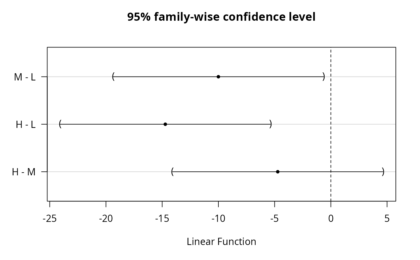
  ### 95% simultaneous confidence intervals
  plot(print(confint(wht)))
#> 
#> 	 Simultaneous Confidence Intervals
#> 
#> Multiple Comparisons of Means: Tukey Contrasts
#> 
#> 
#> Fit: aov(formula = breaks ~ wool + tension, data = warpbreaks)
#> 
#> Quantile = 2.4149
#> 95% family-wise confidence level
#>  
#> 
#> Linear Hypotheses:
#>            Estimate lwr      upr     
#> M - L == 0 -10.0000 -19.3515  -0.6485
#> H - L == 0 -14.7222 -24.0737  -5.3707
#> H - M == 0  -4.7222 -14.0737   4.6293
#> 


  ### the same (for balanced designs only)
  TukeyHSD(amod, "tension")
#>   Tukey multiple comparisons of means
#>     95% family-wise confidence level
#> 
#> Fit: aov(formula = breaks ~ wool + tension, data = warpbreaks)
#> 
#> $tension
#>           diff       lwr        upr     p adj
#> M-L -10.000000 -19.35342 -0.6465793 0.0336262
#> H-L -14.722222 -24.07564 -5.3688015 0.0011218
#> H-M  -4.722222 -14.07564  4.6311985 0.4474210
#> 

  ### corresponding adjusted p values
  summary(wht)
#> 
#> 	 Simultaneous Tests for General Linear Hypotheses
#> 
#> Multiple Comparisons of Means: Tukey Contrasts
#> 
#> 
#> Fit: aov(formula = breaks ~ wool + tension, data = warpbreaks)
#> 
#> Linear Hypotheses:
#>            Estimate Std. Error t value Pr(>|t|)   
#> M - L == 0  -10.000      3.872  -2.582  0.03356 * 
#> H - L == 0  -14.722      3.872  -3.802  0.00114 **
#> H - M == 0   -4.722      3.872  -1.219  0.44742   
#> ---
#> Signif. codes:  0 ‘***’ 0.001 ‘**’ 0.01 ‘*’ 0.05 ‘.’ 0.1 ‘ ’ 1
#> (Adjusted p values reported -- single-step method)
#> 

  ### all means for levels of `tension'
  amod <- aov(breaks ~ tension, data = warpbreaks)
  glht(amod, linfct = matrix(c(1, 0, 0, 
                               1, 1, 0, 
                               1, 0, 1), byrow = TRUE, ncol = 3))
#> 
#> 	 General Linear Hypotheses
#> 
#> Linear Hypotheses:
#>        Estimate
#> 1 == 0    36.39
#> 2 == 0    26.39
#> 3 == 0    21.67
#> 

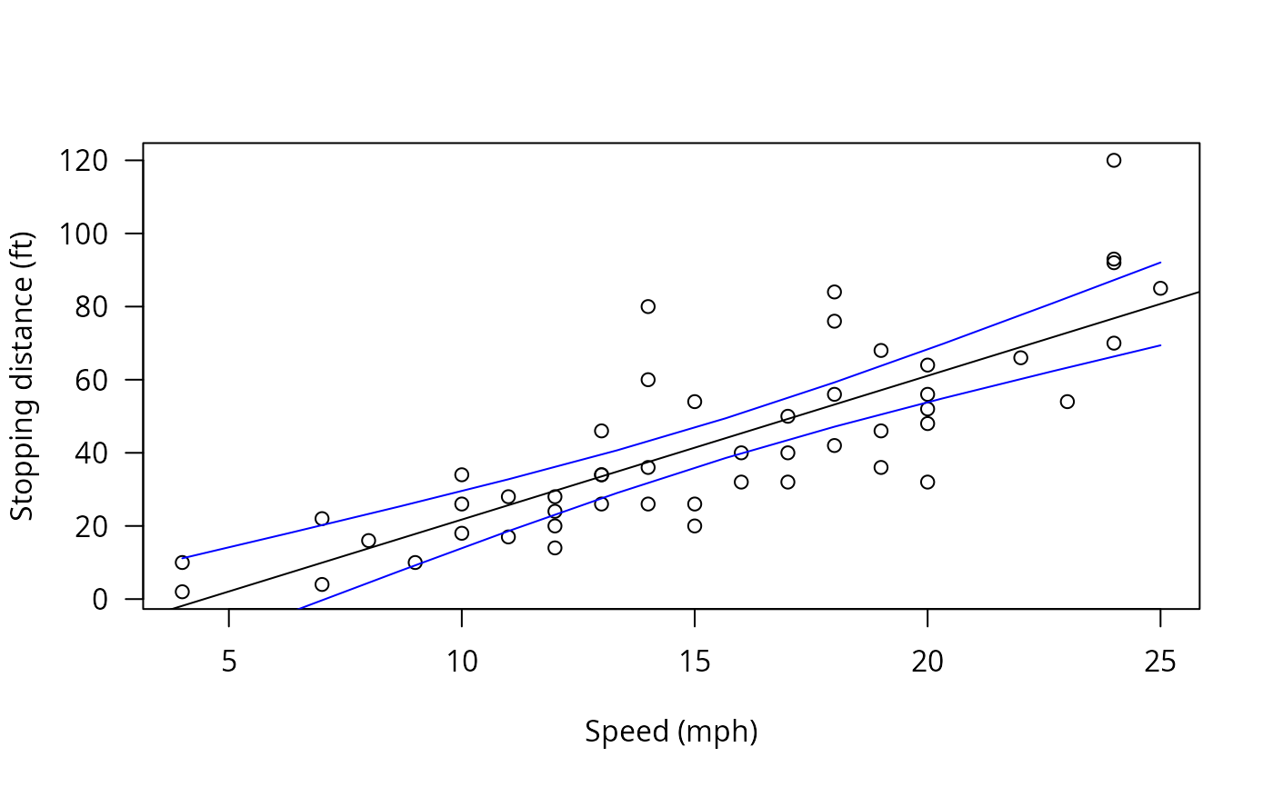
  ### confidence bands for a simple linear model, `cars' data
  plot(cars, xlab = "Speed (mph)", ylab = "Stopping distance (ft)",
       las = 1)

  ### fit linear model and add regression line to plot
  lmod <- lm(dist ~ speed, data = cars)
  abline(lmod)

  ### a grid of speeds
  speeds <- seq(from = min(cars$speed), to = max(cars$speed), 
                length.out = 10)

  ### linear hypotheses: 10 selected points on the regression line != 0
  K <- cbind(1, speeds)                                                        

  ### set up linear hypotheses
  cht <- glht(lmod, linfct = K)

  ### confidence intervals, i.e., confidence bands, and add them plot
  cci <- confint(cht)
  lines(speeds, cci$confint[,"lwr"], col = "blue")
  lines(speeds, cci$confint[,"upr"], col = "blue")



  ### simultaneous p values for parameters in a Cox model
  if (require("survival") && require("MASS")) {
      data("leuk", package = "MASS")
      leuk.cox <- coxph(Surv(time) ~ ag + log(wbc), data = leuk)

      ### set up linear hypotheses
      lht <- glht(leuk.cox, linfct = diag(length(coef(leuk.cox))))

      ### adjusted p values
      print(summary(lht))
  }
#> 
#> 	 Simultaneous Tests for General Linear Hypotheses
#> 
#> Fit: coxph(formula = Surv(time) ~ ag + log(wbc), data = leuk)
#> 
#> Linear Hypotheses:
#>        Estimate Std. Error z value Pr(>|z|)  
#> 1 == 0  -1.0691     0.4293  -2.490   0.0253 *
#> 2 == 0   0.3677     0.1360   2.703   0.0137 *
#> ---
#> Signif. codes:  0 ‘***’ 0.001 ‘**’ 0.01 ‘*’ 0.05 ‘.’ 0.1 ‘ ’ 1
#> (Adjusted p values reported -- single-step method)
#>