Mixed variable optimization using coordinate descent

Usage

mixopt(
  par,
  fn,
  gr = NULL,
  global = "multistart",
  local = "coorddesc",
  ...,
  method,
  verbose = 0,
  track
)

mixopt_blockcd(
  par,
  fn,
  gr = NULL,
  ...,
  control = list(),
  maxblocksize = NULL,
  method,
  fngr = NULL,
  maxiter = 100,
  maxeval = NULL,
  maxtime = NULL,
  verbose = 0,
  track = FALSE
)

mixopt_coorddesc(
  par,
  fn,
  gr = NULL,
  ...,
  method,
  maxiter = 100,
  maxeval = NULL,
  maxtime = NULL,
  verbose = 0,
  track = FALSE
)

mixopt_multistart(
  par,
  fn,
  gr = NULL,
  ...,
  method,
  fngr = NULL,
  n0 = 20,
  n1 = 2,
  maxiter = 100,
  maxeval = NULL,
  verbose = 0,
  groupeval = FALSE,
  track = FALSE
)

Arguments

par: List of parameters
fn: Function to evaluate
gr: Gradient of fn
global: Global optimization algorithm to use. `FALSE` if you only want local optimization.
local: Local optimization algorithm to use.
...: Additional args
method: Optimization method
verbose: How much to print. 0 is none, 1 is standard, 2 is some, 3 is a lot, etc.
track: Should it track the parameters evaluated and value?
control: Parameters for optimizing.
maxblocksize: The maximum number of continuous dimensions that should be placed into a single block.
fngr: Function that returns the function and gradient value for the given input as a list with names "fn" and "gr".
maxiter: Maximum number of outer iterations. For coordinate descent, one iteration is a loop over each parameter.
maxeval: Maximum number of function evaluations. It may go over this number while in an inner optimization loop, but will exit after that.
maxtime: Maximum time to run in seconds. Not an exact limit, only checks occasionally.
n0: For multistart, number of random initial points to evaluate.
n1: For multistart, number of best starts to optimize with. You should have `n0` less than `n1`, potentially by a large factor. gradient descent.
groupeval: Can multiple inputs be evaluated at once? This can speed up greatly for certain circumstances. Use "matrix" to have it give a set of points as rows of a matrix to all be evaluated at once.

Value

List

References

https://en.wikipedia.org/wiki/Coordinate_descent

https://www.uv.es/rmarti/paper/docs/multi2.pdf

Examples

# Simple 1D example
mixopt_blockcd(par=list(mopar_cts(2,8)), fn=function(x) {(4.5-x[1])^2})
#> $par
#> [1] 4.5
#> 
#> $val
#> [1] 0
#> 
#> $counts
#> function gradient 
#>       13        0 
#> 
#> $runtime
#> Time difference of 0.005441189 secs
#> 
# With gradient (isn't faster)
mixopt_blockcd(par=list(mopar_cts(2,8)), fn=function(x) {(4.5-x[1])^2},
               gr=function(x) {-2*(4.5-x[1])})
#> $par
#> [1] 4.5
#> 
#> $val
#> [1] 0
#> 
#> $counts
#> function gradient 
#>        5        4 
#> 
#> $runtime
#> Time difference of 0.0003159046 secs
#> 

# 1D discrete ordered
mixopt_blockcd(par=list(mopar_ordered(100:10000)),
                 fn=function(x) {(x[1] - 500.3)^2})
#> $par
#> [1] 500
#> 
#> $val
#> [1] 0.09
#> 
#> $counts
#> function gradient 
#>       42        0 
#> 
#> $runtime
#> Time difference of 0.0006225109 secs
#> 

# 2D: one continuous, one factor
mixopt_blockcd(par=list(mopar_cts(2,8), mopar_unordered(letters[1:6])),
                 fn=function(x) {ifelse(x[2] == 'b', -1, 0) +
                                 (4.5-x[1])^2})
#> $par
#> mixopt_list: [1] 4.5 b
#> 
#> $val
#> [1] -1
#> 
#> $counts
#> function gradient 
#>       18        0 
#> 
#> $runtime
#> Time difference of 0.0006451607 secs
#> 
# Simple 1D example
mixopt_coorddesc(par=list(mopar_cts(2,8)), fn=function(x) {(4.5-x[1])^2})
#> $par
#> [1] 4.5
#> 
#> $val
#> [1] 0
#> 
#> $counts
#> function gradient 
#>       13        0 
#> 
#> $runtime
#> Time difference of 0.0003259182 secs
#> 

# 1D discrete ordered
mixopt_coorddesc(par=list(mopar_ordered(100:10000)),
                 fn=function(x) {(x[1] - 500.3)^2})
#> $par
#> [1] 500
#> 
#> $val
#> [1] 0.09
#> 
#> $counts
#> function gradient 
#>       42        0 
#> 
#> $runtime
#> Time difference of 0.0006928444 secs
#> 

# 2D: one continuous, one factor
mixopt_coorddesc(par=list(mopar_cts(2,8), mopar_unordered(letters[1:6])),
                 fn=function(x) {ifelse(x[2] == 'b', -1, 0) +
                                 (4.5-x[1])^2})
#> $par
#> mixopt_list: [1] 4.5 b
#> 
#> $val
#> [1] -1
#> 
#> $counts
#> function gradient 
#>       26        0 
#> 
#> $runtime
#> Time difference of 0.001098871 secs
#> 
# 2D
library(ggplot2)
library(dplyr)
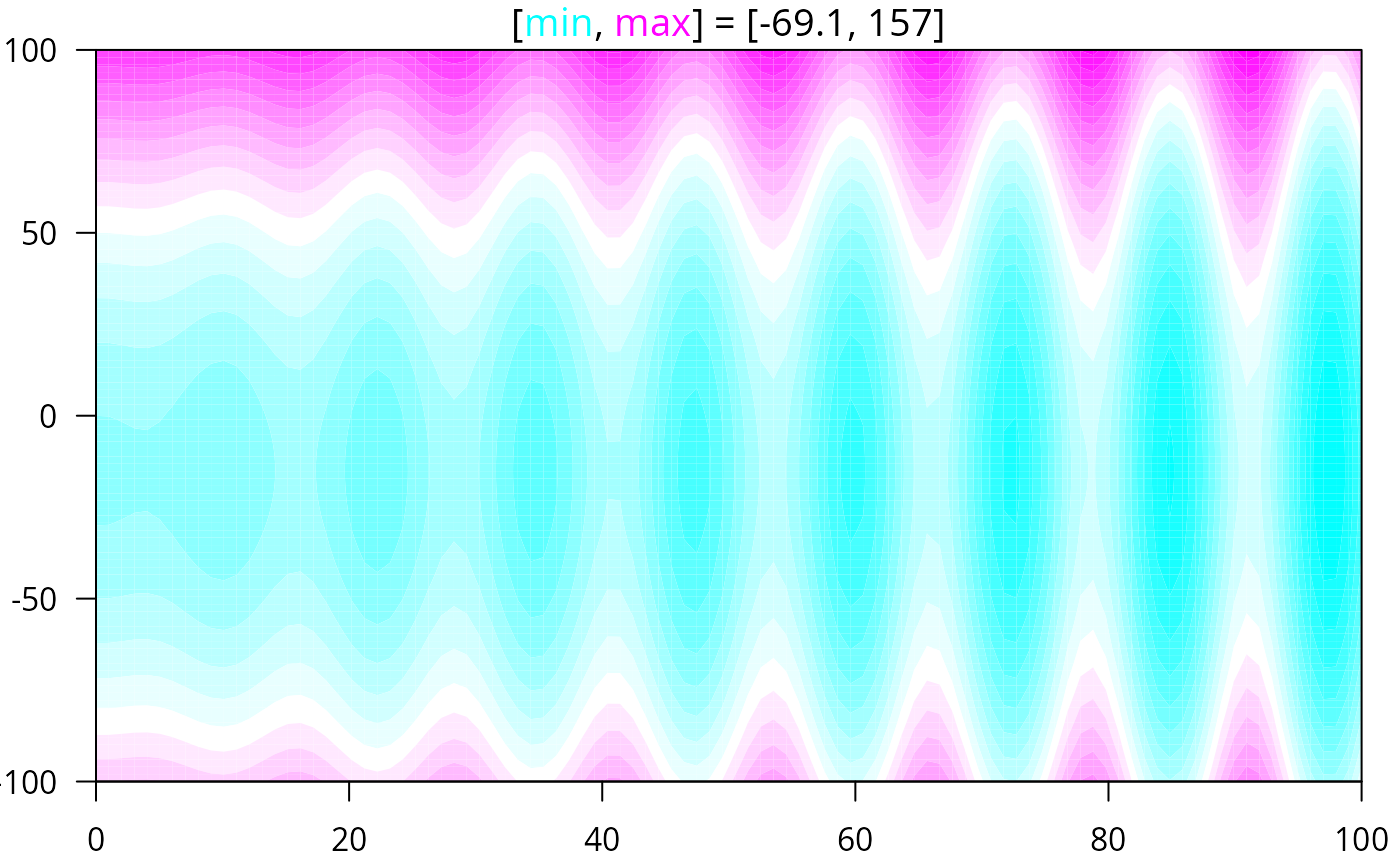
f6 <- function(x) {-(-x[1]*.5*sin(.5*x[1])*1 - 1e-2*x[2]^2 +
                       .2*x[1] - .3*x[2])}

if (requireNamespace("ContourFunctions", quietly = TRUE)) {
  ContourFunctions::cf_func(f6, xlim=c(0,100), ylim=c(-100,100))
}

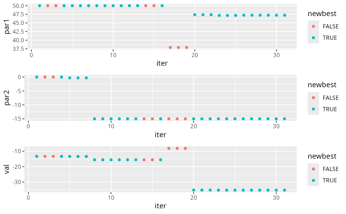
m6 <- mixopt_coorddesc(par=list(mopar_cts(0,100), mopar_cts(-100,100)),
                       fn=f6, track = TRUE)
plot_track(m6)

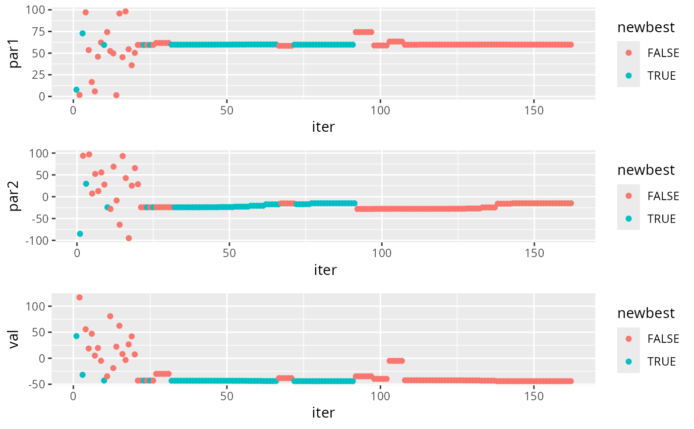
ms6 <- mixopt_multistart(par=list(mopar_cts(0,100), mopar_cts(-100,100)),
                         fn=f6, track = TRUE)
plot_track(ms6)

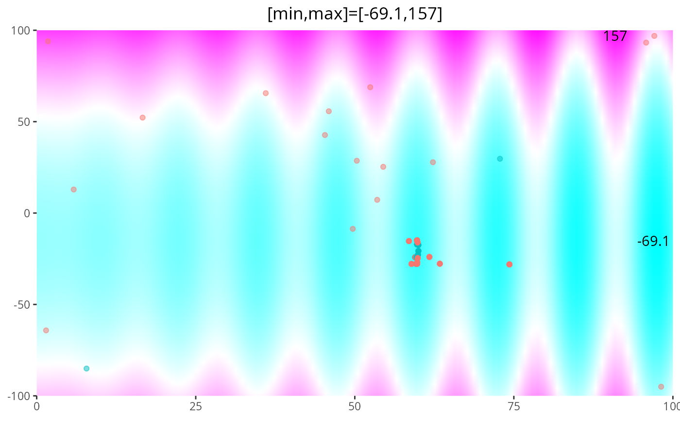
if (requireNamespace("ContourFunctions", quietly = TRUE)) {
  ContourFunctions::cf_func(f6, xlim=c(0,100), ylim=c(-100,100),
                            gg = TRUE) +
    geom_point(data=as.data.frame(matrix(unlist(ms6$track$par),
                                         ncol=2, byrow=TRUE)) %>%
                 bind_cols(newbest=ms6$track$newbest),
               aes(V1, V2, color=newbest), alpha=.5)
}