plot Method for logistf Likelihood Profiles

Provides the plot method for objects created by profile.logistf or CLIP.profile

# S3 method for class 'logistf.profile'
plot(
  x,
  type = "profile",
  max1 = TRUE,
  colmain = "black",
  colimp = "gray",
  plotmain = T,
  ylim = NULL,
  ...
)

Arguments

x

A profile.logistf object

type

Type of plot: one of c("profile", "cdf", "density")

max1

If type="density", normalizes density to maximum 1

colmain

Color for main profile line

colimp

color for completed-data profile lines (for logistf.profile objects that also carry the CLIP.profile class attribute)

plotmain

if FALSE, suppresses the main profile line (for logistf.profile objects that also carry the CLIP.profile class attribute)

ylim

Limits for the y-axis

...

Further arguments to be passed to plot().

Value

The function is called for its side effects

Details

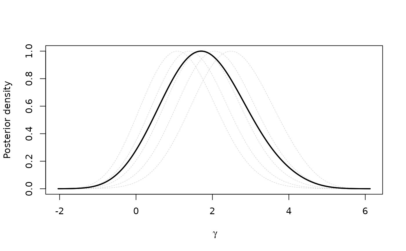
The plot method provides three types of plots (profile, CDF, and density representation of a profile likelihood). For objects generated by CLIP.profile, it also allows to show the completed-data profiles along with the pooled profile.

References

Heinze G, Ploner M, Beyea J (2013). Confidence intervals after multiple imputation: combining profile likelihood information from logistic regressions. Statistics in Medicine, to appear.

Author

Georg Heinze und Meinhard Ploner

Examples

data(sex2) 
fit<-logistf(case ~ age+oc+vic+vicl+vis+dia, data=sex2)
plot(profile(fit,variable="dia"))

plot(profile(fit,variable="dia"), "cdf")

plot(profile(fit,variable="dia"), "density")
#> Warning: Selecting bandwidth *not* using 'weights'


#generate data set with NAs
freq=c(5,2,2,7,5,4)
y<-c(rep(1,freq[1]+freq[2]), rep(0,freq[3]+freq[4]), rep(1,freq[5]), rep(0,freq[6]))
x<-c(rep(1,freq[1]), rep(0,freq[2]), rep(1,freq[3]), rep(0,freq[4]), rep(NA,freq[5]),
   rep(NA,freq[6]))
toy<-data.frame(x=x,y=y)

# impute data set 5 times
set.seed(169)
toymi<-list(0)
for(i in 1:5){
   toymi[[i]]<-toy
   y1<-toymi[[i]]$y==1 & is.na(toymi[[i]]$x)
   y0<-toymi[[i]]$y==0 & is.na(toymi[[i]]$x)
   xnew1<-rbinom(sum(y1),1,freq[1]/(freq[1]+freq[2]))
   xnew0<-rbinom(sum(y0),1,freq[3]/(freq[3]+freq[4]))
   toymi[[i]]$x[y1==TRUE]<-xnew1
   toymi[[i]]$x[y0==TRUE]<-xnew0
 }
 
# logistf analyses of each imputed data set
fit.list<-lapply(1:5, function(X) logistf(data=toymi[[X]], y~x, pl=TRUE))

# CLIP profile 
xprof<-CLIP.profile(obj=fit.list, variable="x", data=toymi, keep=TRUE)
plot(xprof)


#plot as CDF
plot(xprof, "cdf")


#plot as density
plot(xprof, "density")
#> Warning: Selecting bandwidth *not* using 'weights'
#> Warning: Selecting bandwidth *not* using 'weights'
#> Warning: Selecting bandwidth *not* using 'weights'
#> Warning: Selecting bandwidth *not* using 'weights'
#> Warning: Selecting bandwidth *not* using 'weights'
#> Warning: Selecting bandwidth *not* using 'weights'