Model II regression
lmodel2.RdThis function computes model II simple linear regression using the following methods: ordinary least squares (OLS), major axis (MA), standard major axis (SMA), and ranged major axis (RMA). The model only accepts one response and one explanatory variable.
lmodel2(formula, data = NULL, range.y=NULL, range.x=NULL, nperm=0)Arguments
- formula
- data
A data frame containing the two variables specified in the formula.
- range.y, range.x
Parametres for ranged major axis regression (RMA). If
range.y = NULLandrange.x = NULL, RMA will not be computed. If only one of them isNULL, the program will stop. Ifrange.y = "relative": variableyhas a true zero (relative-scale variable). Ifrange.y = "interval": variableypossibly includes negative values (interval-scale variable). Ifrange.x = "relative": variablexhas a true zero (relative-scale variable). Ifrange.x = "interval": variablexpossibly includes negative values (interval-scale variable)- nperm
Number of permutations for the tests. If
nperm =
   0
, tests will not be computed.
Details
Model II regression should be used when the two variables in the
regression equation are random, i.e. not controlled by the
researcher. Model I regression using least squares underestimates
the slope of the linear relationship between the variables when they
both contain error. Ordinary least squares (OLS) is, however, appropriate
in some cases as a model II regression model; see the “Model
II User's guide, R edition” which you can read using command
vignette("mod2user").
The model II regression methods of ordinary least squares (OLS),
major axis (MA), standard major axis (SMA), and ranged major axis
(RMA) are described in Legendre and Legendre (2012, Section
10.3.2). OLS, MA, and SMA are also described in Sokal and Rohlf
(1995). The PDF document “Model II User's guide, R edition”
provided with this function contains a tutorial for model II
regression, and can be read with command
vignette("mod2user").
The plot function plots the data points together with one of the
regression lines, specified by method="OLS", method="MA" (default),
method="SMA", or method="RMA", and its 95 percent confidence interval.
Value
The default output provides the regression output. It draws
information from a list, produced by function lmodel2, which
contains the following elements:
- y
The response variable.
- x
The explanatory variable.
- regression.results
A table with rows corresponding to the four regression methods. Column 1 gives the method name, followed by the intercept and slope estimates, the angle between the regression line and the abscissa, and the permutational probability (one-tailed, for the tail corresponding to the sign of the slope estimate).
- confidence.intervals
A table with rows corresponding to the four regression methods. The method name is followed by the parametric 95 the intercept and slope estimates.
- eigenvalues
Eigenvalues of the bivariate dispersion, computed during major axis regression.
- H
The H statistic used for computing the confidence interval of the major axis slope. Notation following Sokal and Rohlf (1995).
- n
Number of objects.
- r
Correlation coefficient.
- rsquare
Coefficient of determination (R-square) of the OLS regression.
- P.param
2-tailed parametric P-value for the test of r and the OLS slope.
- theta
Angle between the two OLS regression lines,
lm(y ~ x)andlm(x ~ y).- nperm
Number of permutations for the permutation tests.
- epsilon
Any value smaller than epsilon is considered to be zero.
- info.slope
Information about the slope notation when \(r = 0\).
- info.CI
Information about the confidence limits notation when the slope is infinite.
- call
Call of the function.
References
Legendre, P. and L. Legendre. 2012. Numerical ecology, 3rd English edition. Elsevier Science BV, Amsterdam.
Sokal, R. R. and F. J. Rohlf. 1995. Biometry – The principles and practice of statistics in biological research. 3rd edition. W. H. Freeman, New York.
See also
A tutorial (file “Model II User's guide, R edition”) is provided
with this function, and can be read within R session using command
vignette("mod2user", package="lmodel2").
Note
The package exports only the main functions lmodel2,
plot.lmodel2 and lines.lmodel2. Much of the work is
done by internal functions which are not directly visible, but you
can use triple colon to see or directly use these functions (e.g.,
lmodel2:::print.lmodel2). Internal functions that perform
essential parts of the analysis are MA.reg, SMA.reg,
CLma, CLsma and permutest.lmodel2.
Examples
## The example data files are described in more detail in the
## \dQuote{Model II User's guide, R edition} tutorial.
## Example 1 (surgical unit data)
data(mod2ex1)
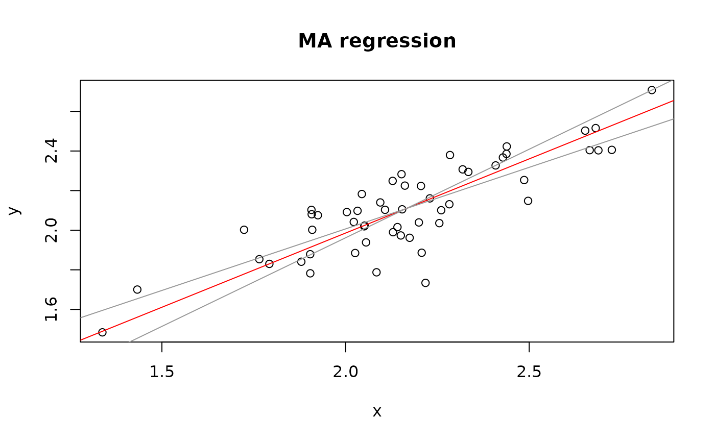
Ex1.res <- lmodel2(Predicted_by_model ~ Survival, data=mod2ex1, nperm=99)
#> RMA was not requested: it will not be computed.
Ex1.res
#>
#> Model II regression
#>
#> Call: lmodel2(formula = Predicted_by_model ~ Survival, data = mod2ex1,
#> nperm = 99)
#>
#> n = 54 r = 0.8387315 r-square = 0.7034705
#> Parametric P-values: 2-tailed = 2.447169e-15 1-tailed = 1.223585e-15
#> Angle between the two OLS regression lines = 9.741174 degrees
#>
#> Permutation tests of OLS, MA, RMA slopes: 1-tailed, tail corresponding to sign
#> A permutation test of r is equivalent to a permutation test of the OLS slope
#> P-perm for SMA = NA because the SMA slope cannot be tested
#>
#> Regression results
#> Method Intercept Slope Angle (degrees) P-perm (1-tailed)
#> 1 OLS 0.6852956 0.6576961 33.33276 0.01
#> 2 MA 0.4871990 0.7492103 36.84093 0.01
#> 3 SMA 0.4115541 0.7841557 38.10197 NA
#>
#> Confidence intervals
#> Method 2.5%-Intercept 97.5%-Intercept 2.5%-Slope 97.5%-Slope
#> 1 OLS 0.4256885 0.9449028 0.5388717 0.7765204
#> 2 MA 0.1725753 0.7633080 0.6216569 0.8945561
#> 3 SMA 0.1349629 0.6493905 0.6742831 0.9119318
#>
#> Eigenvalues: 0.1332385 0.01090251
#>
#> H statistic used for computing C.I. of MA: 0.007515993
#>
plot(Ex1.res)
 ## Example 2 (eagle rays and Macomona)
data(mod2ex2)
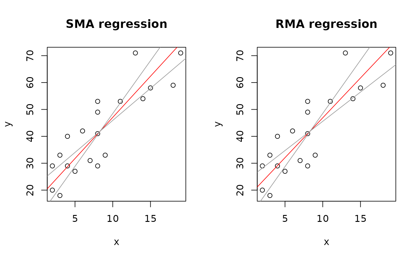
Ex2.res <- lmodel2(Prey ~ Predators, data=mod2ex2, "relative", "relative", 99)
Ex2.res
#>
#> Model II regression
#>
#> Call: lmodel2(formula = Prey ~ Predators, data = mod2ex2, range.y =
#> "relative", range.x = "relative", nperm = 99)
#>
#> n = 20 r = 0.8600787 r-square = 0.7397354
#> Parametric P-values: 2-tailed = 1.161748e-06 1-tailed = 5.808741e-07
#> Angle between the two OLS regression lines = 5.106227 degrees
#>
#> Permutation tests of OLS, MA, RMA slopes: 1-tailed, tail corresponding to sign
#> A permutation test of r is equivalent to a permutation test of the OLS slope
#> P-perm for SMA = NA because the SMA slope cannot be tested
#>
#> Regression results
#> Method Intercept Slope Angle (degrees) P-perm (1-tailed)
#> 1 OLS 20.02675 2.631527 69.19283 0.01
#> 2 MA 13.05968 3.465907 73.90584 0.01
#> 3 SMA 16.45205 3.059635 71.90073 NA
#> 4 RMA 17.25651 2.963292 71.35239 0.01
#>
#> Confidence intervals
#> Method 2.5%-Intercept 97.5%-Intercept 2.5%-Slope 97.5%-Slope
#> 1 OLS 12.490993 27.56251 1.858578 3.404476
#> 2 MA 1.347422 19.76310 2.663101 4.868572
#> 3 SMA 9.195287 22.10353 2.382810 3.928708
#> 4 RMA 8.962997 23.84493 2.174260 3.956527
#>
#> Eigenvalues: 269.8212 6.418234
#>
#> H statistic used for computing C.I. of MA: 0.006120651
#>
op <- par(mfrow = c(1,2))
plot(Ex2.res, "SMA")
plot(Ex2.res, "RMA")
## Example 2 (eagle rays and Macomona)
data(mod2ex2)
Ex2.res <- lmodel2(Prey ~ Predators, data=mod2ex2, "relative", "relative", 99)
Ex2.res
#>
#> Model II regression
#>
#> Call: lmodel2(formula = Prey ~ Predators, data = mod2ex2, range.y =
#> "relative", range.x = "relative", nperm = 99)
#>
#> n = 20 r = 0.8600787 r-square = 0.7397354
#> Parametric P-values: 2-tailed = 1.161748e-06 1-tailed = 5.808741e-07
#> Angle between the two OLS regression lines = 5.106227 degrees
#>
#> Permutation tests of OLS, MA, RMA slopes: 1-tailed, tail corresponding to sign
#> A permutation test of r is equivalent to a permutation test of the OLS slope
#> P-perm for SMA = NA because the SMA slope cannot be tested
#>
#> Regression results
#> Method Intercept Slope Angle (degrees) P-perm (1-tailed)
#> 1 OLS 20.02675 2.631527 69.19283 0.01
#> 2 MA 13.05968 3.465907 73.90584 0.01
#> 3 SMA 16.45205 3.059635 71.90073 NA
#> 4 RMA 17.25651 2.963292 71.35239 0.01
#>
#> Confidence intervals
#> Method 2.5%-Intercept 97.5%-Intercept 2.5%-Slope 97.5%-Slope
#> 1 OLS 12.490993 27.56251 1.858578 3.404476
#> 2 MA 1.347422 19.76310 2.663101 4.868572
#> 3 SMA 9.195287 22.10353 2.382810 3.928708
#> 4 RMA 8.962997 23.84493 2.174260 3.956527
#>
#> Eigenvalues: 269.8212 6.418234
#>
#> H statistic used for computing C.I. of MA: 0.006120651
#>
op <- par(mfrow = c(1,2))
plot(Ex2.res, "SMA")
plot(Ex2.res, "RMA")
 par(op)
## Example 3 (cabezon spawning)
op <- par(mfrow = c(1,2))
data(mod2ex3)
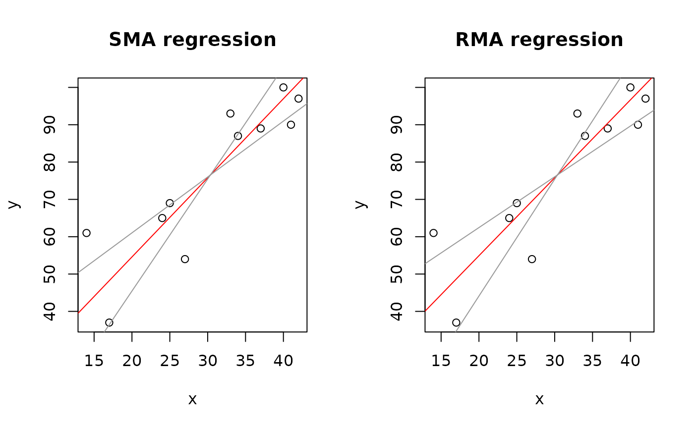
Ex3.res <- lmodel2(No_eggs ~ Mass, data=mod2ex3, "relative", "relative", 99)
Ex3.res
#>
#> Model II regression
#>
#> Call: lmodel2(formula = No_eggs ~ Mass, data = mod2ex3, range.y =
#> "relative", range.x = "relative", nperm = 99)
#>
#> n = 11 r = 0.882318 r-square = 0.7784851
#> Parametric P-values: 2-tailed = 0.0003241737 1-tailed = 0.0001620869
#> Angle between the two OLS regression lines = 5.534075 degrees
#>
#> Permutation tests of OLS, MA, RMA slopes: 1-tailed, tail corresponding to sign
#> A permutation test of r is equivalent to a permutation test of the OLS slope
#> P-perm for SMA = NA because the SMA slope cannot be tested
#>
#> Regression results
#> Method Intercept Slope Angle (degrees) P-perm (1-tailed)
#> 1 OLS 19.766816 1.869955 61.86337 0.01
#> 2 MA 6.656633 2.301728 66.51716 0.01
#> 3 SMA 12.193785 2.119366 64.74023 NA
#> 4 RMA 13.179672 2.086897 64.39718 0.01
#>
#> Confidence intervals
#> Method 2.5%-Intercept 97.5%-Intercept 2.5%-Slope 97.5%-Slope
#> 1 OLS -4.098376 43.63201 1.117797 2.622113
#> 2 MA -36.540814 27.83295 1.604304 3.724398
#> 3 SMA -14.576929 31.09957 1.496721 3.001037
#> 4 RMA -18.475744 35.25317 1.359925 3.129441
#>
#> Eigenvalues: 494.634 17.49327
#>
#> H statistic used for computing C.I. of MA: 0.02161051
#>
plot(Ex3.res, "SMA")
plot(Ex3.res, "RMA")
par(op)
## Example 3 (cabezon spawning)
op <- par(mfrow = c(1,2))
data(mod2ex3)
Ex3.res <- lmodel2(No_eggs ~ Mass, data=mod2ex3, "relative", "relative", 99)
Ex3.res
#>
#> Model II regression
#>
#> Call: lmodel2(formula = No_eggs ~ Mass, data = mod2ex3, range.y =
#> "relative", range.x = "relative", nperm = 99)
#>
#> n = 11 r = 0.882318 r-square = 0.7784851
#> Parametric P-values: 2-tailed = 0.0003241737 1-tailed = 0.0001620869
#> Angle between the two OLS regression lines = 5.534075 degrees
#>
#> Permutation tests of OLS, MA, RMA slopes: 1-tailed, tail corresponding to sign
#> A permutation test of r is equivalent to a permutation test of the OLS slope
#> P-perm for SMA = NA because the SMA slope cannot be tested
#>
#> Regression results
#> Method Intercept Slope Angle (degrees) P-perm (1-tailed)
#> 1 OLS 19.766816 1.869955 61.86337 0.01
#> 2 MA 6.656633 2.301728 66.51716 0.01
#> 3 SMA 12.193785 2.119366 64.74023 NA
#> 4 RMA 13.179672 2.086897 64.39718 0.01
#>
#> Confidence intervals
#> Method 2.5%-Intercept 97.5%-Intercept 2.5%-Slope 97.5%-Slope
#> 1 OLS -4.098376 43.63201 1.117797 2.622113
#> 2 MA -36.540814 27.83295 1.604304 3.724398
#> 3 SMA -14.576929 31.09957 1.496721 3.001037
#> 4 RMA -18.475744 35.25317 1.359925 3.129441
#>
#> Eigenvalues: 494.634 17.49327
#>
#> H statistic used for computing C.I. of MA: 0.02161051
#>
plot(Ex3.res, "SMA")
plot(Ex3.res, "RMA")
 par(op)
## Example 4 (highly correlated random variables)
op <- par(mfrow=c(1,2))
data(mod2ex4)
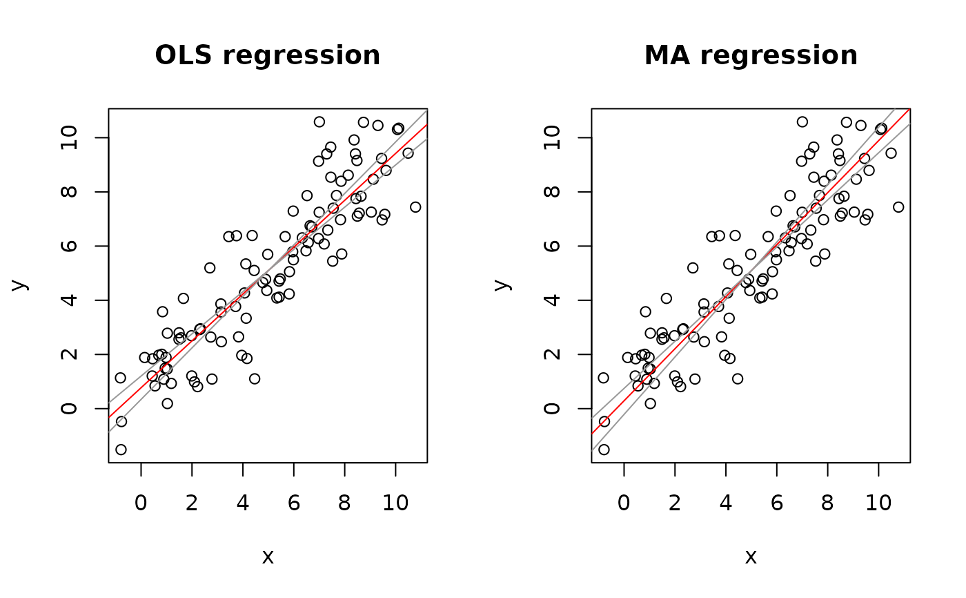
Ex4.res <- lmodel2(y ~ x, data=mod2ex4, "interval", "interval", 99)
Ex4.res
#>
#> Model II regression
#>
#> Call: lmodel2(formula = y ~ x, data = mod2ex4, range.y = "interval",
#> range.x = "interval", nperm = 99)
#>
#> n = 100 r = 0.896898 r-square = 0.804426
#> Parametric P-values: 2-tailed = 1.681417e-36 1-tailed = 8.407083e-37
#> Angle between the two OLS regression lines = 6.218194 degrees
#>
#> Permutation tests of OLS, MA, RMA slopes: 1-tailed, tail corresponding to sign
#> A permutation test of r is equivalent to a permutation test of the OLS slope
#> P-perm for SMA = NA because the SMA slope cannot be tested
#>
#> Regression results
#> Method Intercept Slope Angle (degrees) P-perm (1-tailed)
#> 1 OLS 0.7713474 0.8648893 40.85618 0.01
#> 2 MA 0.2905866 0.9602938 43.83962 0.01
#> 3 SMA 0.2703395 0.9643118 43.95915 NA
#> 4 RMA 0.3142417 0.9555996 43.69937 0.01
#>
#> Confidence intervals
#> Method 2.5%-Intercept 97.5%-Intercept 2.5%-Slope 97.5%-Slope
#> 1 OLS 0.2663618 1.2763329 0.7794015 0.950377
#> 2 MA -0.2121756 0.7477724 0.8695676 1.060064
#> 3 SMA -0.1795065 0.6820701 0.8826059 1.053581
#> 4 RMA -0.1848274 0.7702125 0.8651145 1.054637
#>
#> Eigenvalues: 17.56697 0.9534124
#>
#> H statistic used for computing C.I. of MA: 0.002438452
#>
plot(Ex4.res, "OLS")
plot(Ex4.res, "MA")
par(op)
## Example 4 (highly correlated random variables)
op <- par(mfrow=c(1,2))
data(mod2ex4)
Ex4.res <- lmodel2(y ~ x, data=mod2ex4, "interval", "interval", 99)
Ex4.res
#>
#> Model II regression
#>
#> Call: lmodel2(formula = y ~ x, data = mod2ex4, range.y = "interval",
#> range.x = "interval", nperm = 99)
#>
#> n = 100 r = 0.896898 r-square = 0.804426
#> Parametric P-values: 2-tailed = 1.681417e-36 1-tailed = 8.407083e-37
#> Angle between the two OLS regression lines = 6.218194 degrees
#>
#> Permutation tests of OLS, MA, RMA slopes: 1-tailed, tail corresponding to sign
#> A permutation test of r is equivalent to a permutation test of the OLS slope
#> P-perm for SMA = NA because the SMA slope cannot be tested
#>
#> Regression results
#> Method Intercept Slope Angle (degrees) P-perm (1-tailed)
#> 1 OLS 0.7713474 0.8648893 40.85618 0.01
#> 2 MA 0.2905866 0.9602938 43.83962 0.01
#> 3 SMA 0.2703395 0.9643118 43.95915 NA
#> 4 RMA 0.3142417 0.9555996 43.69937 0.01
#>
#> Confidence intervals
#> Method 2.5%-Intercept 97.5%-Intercept 2.5%-Slope 97.5%-Slope
#> 1 OLS 0.2663618 1.2763329 0.7794015 0.950377
#> 2 MA -0.2121756 0.7477724 0.8695676 1.060064
#> 3 SMA -0.1795065 0.6820701 0.8826059 1.053581
#> 4 RMA -0.1848274 0.7702125 0.8651145 1.054637
#>
#> Eigenvalues: 17.56697 0.9534124
#>
#> H statistic used for computing C.I. of MA: 0.002438452
#>
plot(Ex4.res, "OLS")
plot(Ex4.res, "MA")
 par(op)
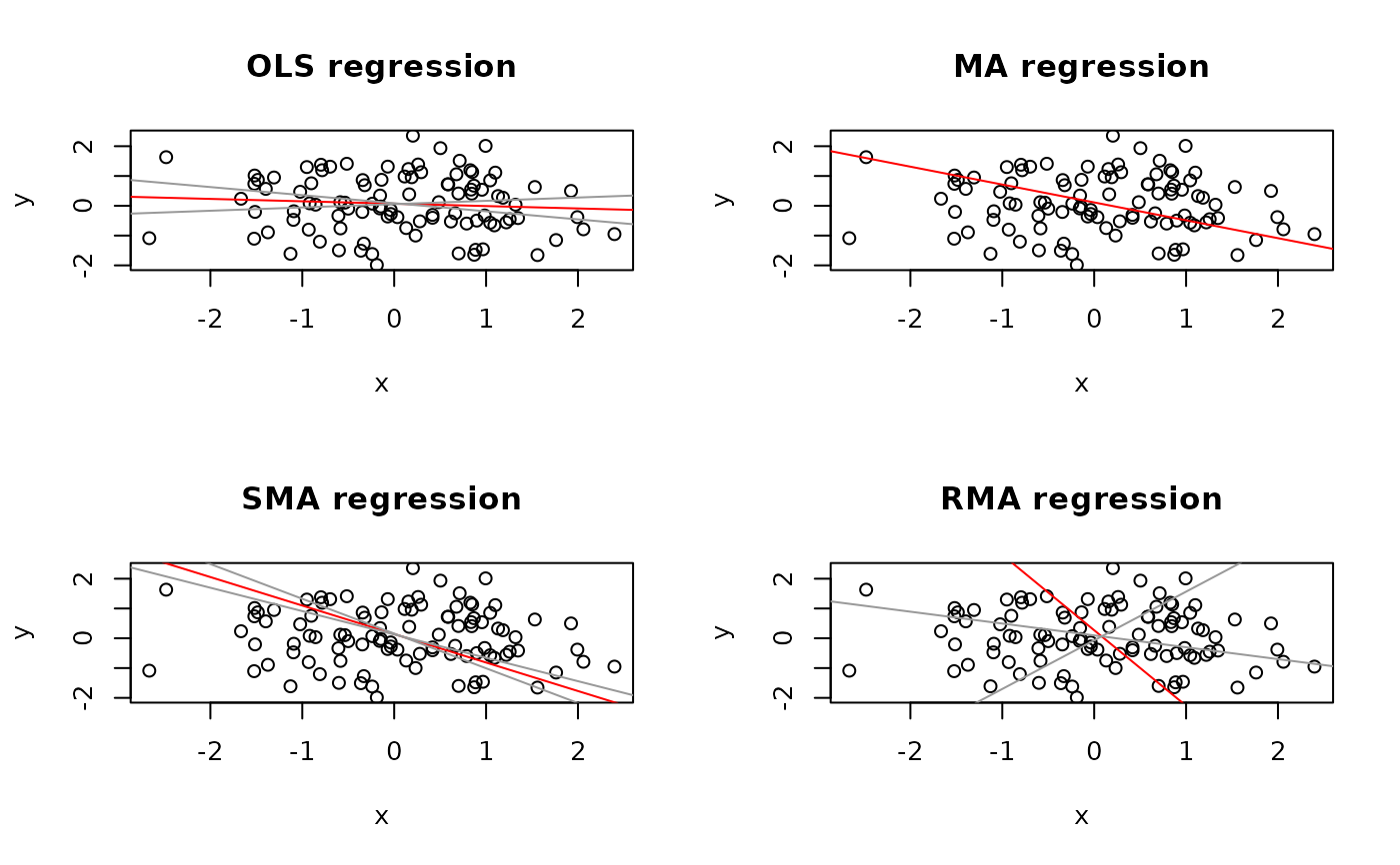
# Example 5 (uncorrelated random variables)
data(mod2ex5)
Ex5.res <- lmodel2(random_y ~ random_x, data=mod2ex5, "interval", "interval", 99)
Ex5.res
#>
#> Model II regression
#>
#> Call: lmodel2(formula = random_y ~ random_x, data = mod2ex5, range.y =
#> "interval", range.x = "interval", nperm = 99)
#>
#> n = 100 r = -0.0837681 r-square = 0.007017094
#> Parametric P-values: 2-tailed = 0.4073269 1-tailed = 0.2036634
#> Angle between the two OLS regression lines = 80.41387 degrees
#>
#> Permutation tests of OLS, MA, RMA slopes: 1-tailed, tail corresponding to sign
#> A permutation test of r is equivalent to a permutation test of the OLS slope
#> P-perm for SMA = NA because the SMA slope cannot be tested
#>
#> Confidence interval = NA when the limits of the confidence interval
#> cannot be computed. This happens when the correlation is 0
#> or the C.I. includes all 360 deg. of the plane (H >= 1)
#>
#> Regression results
#> Method Intercept Slope Angle (degrees) P-perm (1-tailed)
#> 1 OLS 0.07074386 -0.08010978 -4.580171 0.18
#> 2 MA 0.11293376 -0.60004584 -30.965688 0.18
#> 3 SMA 0.14184407 -0.95632810 -43.721176 NA
#> 4 RMA 0.26977945 -2.53296649 -68.456190 0.18
#>
#> Confidence intervals
#> Method 2.5%-Intercept 97.5%-Intercept 2.5%-Slope 97.5%-Slope
#> 1 OLS -0.1220525 0.26354020 -0.2711429 0.1109234
#> 2 MA NA NA NA NA
#> 3 SMA 0.1278759 0.15887844 -1.1662547 -0.7841884
#> 4 RMA 0.0965427 -0.06826575 1.6330043 -0.3980472
#>
#> Eigenvalues: 1.071318 0.8857145
#>
#> H statistic used for computing C.I. of MA: 1.106884
#>
op <- par(mfrow = c(2,2))
plot(Ex5.res, "OLS")
plot(Ex5.res, "MA")
plot(Ex5.res, "SMA")
plot(Ex5.res, "RMA")
par(op)
# Example 5 (uncorrelated random variables)
data(mod2ex5)
Ex5.res <- lmodel2(random_y ~ random_x, data=mod2ex5, "interval", "interval", 99)
Ex5.res
#>
#> Model II regression
#>
#> Call: lmodel2(formula = random_y ~ random_x, data = mod2ex5, range.y =
#> "interval", range.x = "interval", nperm = 99)
#>
#> n = 100 r = -0.0837681 r-square = 0.007017094
#> Parametric P-values: 2-tailed = 0.4073269 1-tailed = 0.2036634
#> Angle between the two OLS regression lines = 80.41387 degrees
#>
#> Permutation tests of OLS, MA, RMA slopes: 1-tailed, tail corresponding to sign
#> A permutation test of r is equivalent to a permutation test of the OLS slope
#> P-perm for SMA = NA because the SMA slope cannot be tested
#>
#> Confidence interval = NA when the limits of the confidence interval
#> cannot be computed. This happens when the correlation is 0
#> or the C.I. includes all 360 deg. of the plane (H >= 1)
#>
#> Regression results
#> Method Intercept Slope Angle (degrees) P-perm (1-tailed)
#> 1 OLS 0.07074386 -0.08010978 -4.580171 0.18
#> 2 MA 0.11293376 -0.60004584 -30.965688 0.18
#> 3 SMA 0.14184407 -0.95632810 -43.721176 NA
#> 4 RMA 0.26977945 -2.53296649 -68.456190 0.18
#>
#> Confidence intervals
#> Method 2.5%-Intercept 97.5%-Intercept 2.5%-Slope 97.5%-Slope
#> 1 OLS -0.1220525 0.26354020 -0.2711429 0.1109234
#> 2 MA NA NA NA NA
#> 3 SMA 0.1278759 0.15887844 -1.1662547 -0.7841884
#> 4 RMA 0.0965427 -0.06826575 1.6330043 -0.3980472
#>
#> Eigenvalues: 1.071318 0.8857145
#>
#> H statistic used for computing C.I. of MA: 1.106884
#>
op <- par(mfrow = c(2,2))
plot(Ex5.res, "OLS")
plot(Ex5.res, "MA")
plot(Ex5.res, "SMA")
plot(Ex5.res, "RMA")
 par(op)
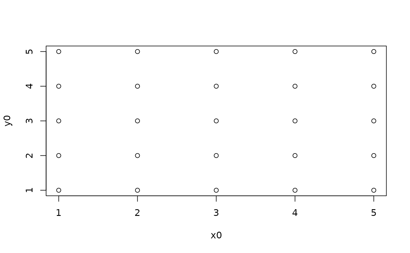
## Example 6 where cor(y,x) = 0 by construct (square grid of points)
y0 = rep(c(1,2,3,4,5),5)
x0 = c(rep(1,5),rep(2,5),rep(3,5),rep(4,5),rep(5,5))
plot(x0, y0)
par(op)
## Example 6 where cor(y,x) = 0 by construct (square grid of points)
y0 = rep(c(1,2,3,4,5),5)
x0 = c(rep(1,5),rep(2,5),rep(3,5),rep(4,5),rep(5,5))
plot(x0, y0)
 Ex6 = as.data.frame(cbind(x0,y0))
zero.res = lmodel2(y0 ~ x0, data=Ex6, "relative", "relative")
#> Warning: MA: R-square = 0
#> Warning: SMA: R-square = 0
#> Warning: RMA: R-square = 0
#> No permutation test will be performed
print(zero.res)
#>
#> Model II regression
#>
#> Call: lmodel2(formula = y0 ~ x0, data = Ex6, range.y = "relative",
#> range.x = "relative")
#>
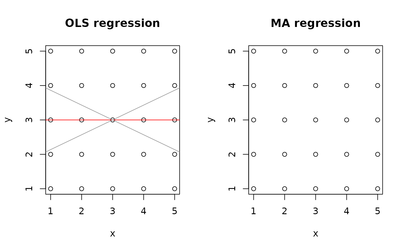
#> n = 25 r = 0 r-square = 0
#> Parametric P-values: 2-tailed = 1 1-tailed = 0.5
#> Angle between the two OLS regression lines = 90 degrees
#> MA, SMA, RMA slopes = NA when the correlation is zero
#>
#> Confidence interval = NA when the limits of the confidence interval
#> cannot be computed. This happens when the correlation is 0
#> or the C.I. includes all 360 deg. of the plane (H >= 1)
#>
#> Regression results
#> Method Intercept Slope Angle (degrees) P-perm (1-tailed)
#> 1 OLS 3 -4.195057e-16 -2.40359e-14 NA
#> 2 MA NA NA NA NA
#> 3 SMA NA NA NA NA
#> 4 RMA NA NA NA NA
#>
#> Confidence intervals
#> Method 2.5%-Intercept 97.5%-Intercept 2.5%-Slope 97.5%-Slope
#> 1 OLS 1.569391 4.430609 -0.4313449 0.4313449
#> 2 MA NA NA NA NA
#> 3 SMA NA NA NA NA
#> 4 RMA NA NA NA NA
#>
#> Eigenvalues: 2.083333 2.083333
#>
#> H statistic used for computing C.I. of MA: NA
#>
op <- par(mfrow = c(1,2))
plot(zero.res, "OLS")
plot(zero.res, "MA")
#> Warning: R-square = 0: model and C.I. not drawn for MA, SMA or RMA
Ex6 = as.data.frame(cbind(x0,y0))
zero.res = lmodel2(y0 ~ x0, data=Ex6, "relative", "relative")
#> Warning: MA: R-square = 0
#> Warning: SMA: R-square = 0
#> Warning: RMA: R-square = 0
#> No permutation test will be performed
print(zero.res)
#>
#> Model II regression
#>
#> Call: lmodel2(formula = y0 ~ x0, data = Ex6, range.y = "relative",
#> range.x = "relative")
#>
#> n = 25 r = 0 r-square = 0
#> Parametric P-values: 2-tailed = 1 1-tailed = 0.5
#> Angle between the two OLS regression lines = 90 degrees
#> MA, SMA, RMA slopes = NA when the correlation is zero
#>
#> Confidence interval = NA when the limits of the confidence interval
#> cannot be computed. This happens when the correlation is 0
#> or the C.I. includes all 360 deg. of the plane (H >= 1)
#>
#> Regression results
#> Method Intercept Slope Angle (degrees) P-perm (1-tailed)
#> 1 OLS 3 -4.195057e-16 -2.40359e-14 NA
#> 2 MA NA NA NA NA
#> 3 SMA NA NA NA NA
#> 4 RMA NA NA NA NA
#>
#> Confidence intervals
#> Method 2.5%-Intercept 97.5%-Intercept 2.5%-Slope 97.5%-Slope
#> 1 OLS 1.569391 4.430609 -0.4313449 0.4313449
#> 2 MA NA NA NA NA
#> 3 SMA NA NA NA NA
#> 4 RMA NA NA NA NA
#>
#> Eigenvalues: 2.083333 2.083333
#>
#> H statistic used for computing C.I. of MA: NA
#>
op <- par(mfrow = c(1,2))
plot(zero.res, "OLS")
plot(zero.res, "MA")
#> Warning: R-square = 0: model and C.I. not drawn for MA, SMA or RMA
 par(op)