Fit Linear Mixed-Effects Models

Fit a linear mixed-effects model (LMM) to data, via restricted maximum likelihood (REML) or maximum likelihood.

Usage

lmer(formula, data = NULL, REML = TRUE, control = lmerControl(),
     start = NULL, verbose = 0L, subset, weights, na.action,
     offset, contrasts = NULL, devFunOnly = FALSE)

Arguments

formula

a two-sided linear formula object describing both the fixed-effects and random-effects part of the model, with the response on the left of a ~ operator and the terms, separated by + operators, on the right. Random-effects terms are distinguished by vertical bars (|) separating expressions for design matrices from grouping factors. By default, non-scalar random effects (where the design matrix has more than one column, e.g. (1+x|f)) are fitted with unstructured (general positive semidefinite) covariance matrices.

Two vertical bars (||) can be used to specify multiple uncorrelated random effects for the same grouping variable. With default settings, the ||-syntax works only for design matrices containing numeric (continuous) predictors; to fit models with independent categorical effects, use diag(f|g) or set options(lme4.doublevert.default = "diag_special") (see getDoublevertDefault).
Tags preceding a random effect term specify covariance structure:
- us (default: us(f|g) is equivalent to (f|g)): unstructured, positive semi-definite
- diag: diagonal (all correlations set to zero). Specify diag(f|g, hom = TRUE) to fit a homogeneous diagonal covariance matrix
- cs: compound symmetric (all pairwise correlations set identical). Specify cs(f|g, hom = TRUE) for homogeneous variances.
- ar1: autoregressive order 1. Note that AR1 models are homogeneous by default; specify ar1(f|g, hom = FALSE) for heterogeneous variances.

data

an optional data frame containing the variables named in formula. By default the variables are taken from the environment from which lmer is called. While data is optional, the package authors strongly recommend its use, especially when later applying methods such as update and drop1 to the fitted model (such methods are not guaranteed to work properly if data is omitted). If data is omitted, variables will be taken from the environment of formula (if specified as a formula) or from the parent frame (if specified as a character vector).

REML

logical scalar - Should the estimates be chosen to optimize the REML criterion (as opposed to the log-likelihood)?

control

a list (of correct class, resulting from lmerControl() or glmerControl() respectively) containing control parameters, including the nonlinear optimizer to be used and parameters to be passed through to the nonlinear optimizer, see the *lmerControl documentation for details.

start

a numeric vector or a named list with optional components, one named par or theta and another named fixef or beta, giving starting values for covariance parameters and fixed effect coefficients, respectively. Specifying start as a numeric vector initializes only the covariance parameters (i.e., it is equivalent to list(par = start), leaving fixed effect parameters at their default starting values (i.e., all zero)). For each term, par/theta specifies the relative covariances of random effects terms, as follows:

for unstructured (us) terms, entries are the lower-triangular elements of the relative Cholesky factor \(\Lambda_\theta\);
for diagonal (diag) terms, entries are the standard deviation parameter(s);
for compound-symmetry (cs) and AR(1) (ar1) terms, entries are the standard deviation parameter(s) followed by the correlation parameter \(\rho\) (specified on the [0,1] scale).

See the covariance structures vignette for more detail on covariance matrix parameterizations.

The parameters for all random-effect terms are concatenated in the starting parameter vector, in the order specified by the internal ordering of the terms. This matches the order in which the terms are returned in VarCorr(), but may not match the order in which the terms are specified in the formula; as noted in the lmer vignette, random effect terms are stored in decreasing order of the number of levels of the grouping variable.

For structured terms, the supplied par values are internally mapped by getTheta() to the corresponding lower-triangular \(\Lambda_\theta\) entries used by the optimizer.

verbose

integer scalar. If > 0 verbose output is generated during the optimization of the parameter estimates. If > 1 verbose output is generated during the individual penalized iteratively reweighted least squares (PIRLS) steps.

subset

an optional expression indicating the subset of the rows of data that should be used in the fit. This can be a logical vector, or a numeric vector indicating which observation numbers are to be included, or a character vector of the row names to be included. All observations are included by default.

weights

an optional vector of ‘prior weights’ to be used in the fitting process. Should be NULL or a numeric vector. Prior weights are not normalized or standardized in any way. In particular, the diagonal of the residual covariance matrix is the squared residual standard deviation parameter sigma times the vector of inverse weights. Therefore, if the weights have relatively large magnitudes, then in order to compensate, the sigma parameter will also need to have a relatively large magnitude.

na.action

a function that indicates what should happen when the data contain NAs. The default action (na.omit, inherited from the 'factory fresh' value of getOption("na.action")) strips any observations with any missing values in any variables.

offset

this can be used to specify an a priori known component to be included in the linear predictor during fitting. This should be NULL or a numeric vector of length equal to the number of cases. One or more offset terms can be included in the formula instead or as well, and if more than one is specified their sum is used. See model.offset.

contrasts

an optional list. See the contrasts.arg of model.matrix.default.

devFunOnly

logical - return only the deviance evaluation function. Note that because the deviance function operates on variables stored in its environment, it may not return exactly the same values on subsequent calls (but the results should always be within machine tolerance).

Value

An object of class merMod (more specifically, an object of subclass lmerMod), for which many methods are available (e.g. methods(class="merMod"))

Note

In earlier version of the lme4 package, a method argument was used. Its functionality has been replaced by the REML argument.

Also, lmer(.) allowed a family argument (to effectively switch to glmer(.)). This has been deprecated in summer 2013, and been disabled in spring 2019.

Details

If the formula argument is specified as a character vector, the function will attempt to coerce it to a formula. However, this is not recommended (users who want to construct formulas by pasting together components are advised to use as.formula or reformulate); model fits will work but subsequent methods such as drop1, update, etc. may fail.
When handling perfectly collinear predictor variables (i.e. fixed-effect design matrices of less than full rank), [gn]lmer is not as sophisticated as modeling frameworks such as lm and glm. While it does automatically drop collinear variables (with a message rather than a warning), it does not automatically fill in NA values for the dropped coefficients; these can be added via fixef(fitted.model, add.dropped=TRUE). This information can also be retrieved via attr(getME(fitted.model, "X"), "col.dropped").
the deviance function returned when devFunOnly is TRUE takes a single numeric vector argument which defines the scaled variance-covariance matrices of the random effects.
- In the case of unstructured covariances, this vector is directly mapped to the theta vector, which represents the unique non-zero values in the Cholesky factor of the (scaled) covariance matrix. For models with only simple (intercept-only) random effects, par (and thus theta) is a vector of the standard deviations of the random effects. For more complex or multiple random effects, running getME(.,"par") or (equivalently) getME(., "theta") to retrieve the theta vector for a fitted model and examining the names of the vector is probably the easiest way to determine the correspondence between the elements of the theta vector and elements of the lower triangles of the Cholesky factors of the random effects.
- For structured covariances, the getTheta method translates the parameter vector to the theta (Cholesky-factor element) scale for internal use. The parameter vector is usually composed of a set of standard-deviation values (one if hom = TRUE or many if hom = FALSE), followed by one or more parameters that determine the correlation matrix.

Examples

## linear mixed models - reference values from older code
(fm1 <- lmer(Reaction ~ Days + (Days | Subject), sleepstudy))
#> Linear mixed model fit by REML ['lmerMod']
#> Formula: Reaction ~ Days + (Days | Subject)
#>    Data: sleepstudy
#> REML criterion at convergence: 1743.628
#> Random effects:
#>  Groups   Name        Std.Dev. Corr 
#>  Subject  (Intercept) 24.741        
#>           Days         5.922   0.07 
#>  Residual             25.592        
#> Number of obs: 180, groups:  Subject, 18
#> Fixed Effects:
#> (Intercept)         Days  
#>      251.41        10.47  
summary(fm1) # (with its own print method; see class?merMod % ./merMod-class.Rd
#> Linear mixed model fit by REML ['lmerMod']
#> Formula: Reaction ~ Days + (Days | Subject)
#>    Data: sleepstudy
#> 
#> REML criterion at convergence: 1743.6
#> 
#> Scaled residuals: 
#>     Min      1Q  Median      3Q     Max 
#> -3.9536 -0.4634  0.0231  0.4634  5.1793 
#> 
#> Random effects:
#>  Groups   Name        Variance Std.Dev. Corr 
#>  Subject  (Intercept) 612.10   24.741        
#>           Days         35.07    5.922   0.07 
#>  Residual             654.94   25.592        
#> Number of obs: 180, groups:  Subject, 18
#> 
#> Fixed effects:
#>             Estimate Std. Error t value
#> (Intercept)  251.405      6.825  36.838
#> Days          10.467      1.546   6.771
#> 
#> Correlation of Fixed Effects:
#>      (Intr)
#> Days -0.138
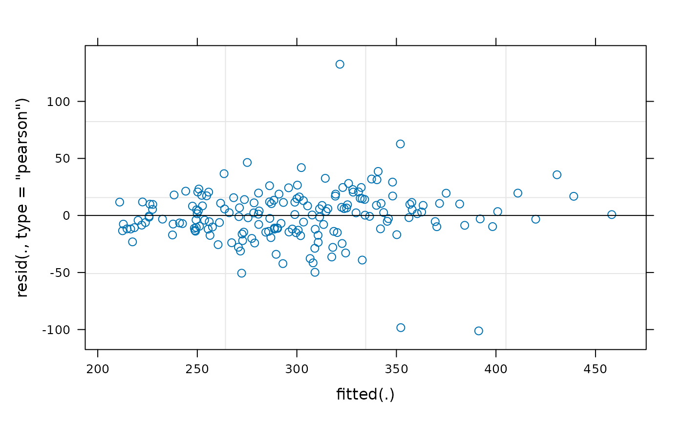
plot(fm1) # plotting the model diagnostics; see ?plot.merMod


str(terms(fm1))
#> Classes 'terms', 'formula'  language Reaction ~ Days
#>   ..- attr(*, "variables")= language list(Reaction, Days)
#>   ..- attr(*, "factors")= int [1:2, 1] 0 1
#>   .. ..- attr(*, "dimnames")=List of 2
#>   .. .. ..$ : chr [1:2] "Reaction" "Days"
#>   .. .. ..$ : chr "Days"
#>   ..- attr(*, "term.labels")= chr "Days"
#>   ..- attr(*, "order")= int 1
#>   ..- attr(*, "intercept")= int 1
#>   ..- attr(*, "response")= int 1
#>   ..- attr(*, ".Environment")=<environment: 0x55f37e889668> 
#>   ..- attr(*, "predvars")= language list(Reaction, Days)
stopifnot(identical(terms(fm1, fixed.only=FALSE),
                    terms(model.frame(fm1))))
attr(terms(fm1, FALSE), "dataClasses") # fixed.only=FALSE needed for dataCl.
#>  Reaction      Days   Subject 
#> "numeric" "numeric"  "factor" 

## Maximum Likelihood (ML), and "monitor" iterations via 'verbose':
fm1_ML <- update(fm1, REML=FALSE, verbose = 1)
#> iteration: 1
#> 	f(x) = 1784.642296
#> iteration: 2
#> 	f(x) = 1790.125637
#> iteration: 3
#> 	f(x) = 1798.999624
#> iteration: 4
#> 	f(x) = 1803.853200
#> iteration: 5
#> 	f(x) = 1800.613981
#> iteration: 6
#> 	f(x) = 1798.604631
#> iteration: 7
#> 	f(x) = 1752.260737
#> iteration: 8
#> 	f(x) = 1797.587692
#> iteration: 9
#> 	f(x) = 1754.954110
#> iteration: 10
#> 	f(x) = 1753.695682
#> iteration: 11
#> 	f(x) = 1754.816999
#> iteration: 12
#> 	f(x) = 1753.106734
#> iteration: 13
#> 	f(x) = 1752.939377
#> iteration: 14
#> 	f(x) = 1752.256879
#> iteration: 15
#> 	f(x) = 1752.057448
#> iteration: 16
#> 	f(x) = 1752.022389
#> iteration: 17
#> 	f(x) = 1752.022728
#> iteration: 18
#> 	f(x) = 1751.971687
#> iteration: 19
#> 	f(x) = 1751.952603
#> iteration: 20
#> 	f(x) = 1751.948524
#> iteration: 21
#> 	f(x) = 1751.987176
#> iteration: 22
#> 	f(x) = 1751.983213
#> iteration: 23
#> 	f(x) = 1751.951971
#> iteration: 24
#> 	f(x) = 1751.946276
#> iteration: 25
#> 	f(x) = 1751.946698
#> iteration: 26
#> 	f(x) = 1751.947568
#> iteration: 27
#> 	f(x) = 1751.945312
#> iteration: 28
#> 	f(x) = 1751.944180
#> iteration: 29
#> 	f(x) = 1751.943533
#> iteration: 30
#> 	f(x) = 1751.942441
#> iteration: 31
#> 	f(x) = 1751.942170
#> iteration: 32
#> 	f(x) = 1751.942370
#> iteration: 33
#> 	f(x) = 1751.942278
#> iteration: 34
#> 	f(x) = 1751.942204
#> iteration: 35
#> 	f(x) = 1751.941309
#> iteration: 36
#> 	f(x) = 1751.940931
#> iteration: 37
#> 	f(x) = 1751.940567
#> iteration: 38
#> 	f(x) = 1751.940179
#> iteration: 39
#> 	f(x) = 1751.940082
#> iteration: 40
#> 	f(x) = 1751.940270
#> iteration: 41
#> 	f(x) = 1751.941501
#> iteration: 42
#> 	f(x) = 1751.939489
#> iteration: 43
#> 	f(x) = 1751.939392
#> iteration: 44
#> 	f(x) = 1751.939398
#> iteration: 45
#> 	f(x) = 1751.939425
#> iteration: 46
#> 	f(x) = 1751.939355
#> iteration: 47
#> 	f(x) = 1751.939490
#> iteration: 48
#> 	f(x) = 1751.939363
#> iteration: 49
#> 	f(x) = 1751.939345
#> iteration: 50
#> 	f(x) = 1751.939344
#> iteration: 51
#> 	f(x) = 1751.939345
#> iteration: 52
#> 	f(x) = 1751.939348
#> iteration: 53
#> 	f(x) = 1751.939344
(fm2 <- lmer(Reaction ~ Days + (Days || Subject), sleepstudy))
#> Linear mixed model fit by REML ['lmerMod']
#> Formula: Reaction ~ Days + ((1 | Subject) + (0 + Days | Subject))
#>    Data: sleepstudy
#> REML criterion at convergence: 1743.669
#> Random effects:
#>  Groups    Name        Std.Dev.
#>  Subject   (Intercept) 25.051  
#>  Subject.1 Days         5.988  
#>  Residual              25.565  
#> Number of obs: 180, groups:  Subject, 18
#> Fixed Effects:
#> (Intercept)         Days  
#>      251.41        10.47  
anova(fm1, fm2)
#> refitting model(s) with ML (instead of REML)
#> Data: sleepstudy
#> Models:
#> fm2: Reaction ~ Days + ((1 | Subject) + (0 + Days | Subject))
#> fm1: Reaction ~ Days + (Days | Subject)
#>     npar    AIC    BIC  logLik -2*log(L)  Chisq Df Pr(>Chisq)
#> fm2    5 1762.0 1778.0 -876.00    1752.0                     
#> fm1    6 1763.9 1783.1 -875.97    1751.9 0.0639  1     0.8004
sm2 <- summary(fm2)
print(fm2, digits=7, ranef.comp="Var") # the print.merMod()         method
#> Linear mixed model fit by REML ['lmerMod']
#> Formula: Reaction ~ Days + ((1 | Subject) + (0 + Days | Subject))
#>    Data: sleepstudy
#> REML criterion at convergence: 1743.669
#> Random effects:
#>  Groups    Name        Variance 
#>  Subject   (Intercept) 627.56905
#>  Subject.1 Days         35.85838
#>  Residual              653.58350
#> Number of obs: 180, groups:  Subject, 18
#> Fixed Effects:
#> (Intercept)         Days  
#>   251.40510     10.46729  
print(sm2, digits=3, corr=FALSE)       # the print.summary.merMod() method
#> Linear mixed model fit by REML ['lmerMod']
#> Formula: Reaction ~ Days + ((1 | Subject) + (0 + Days | Subject))
#>    Data: sleepstudy
#> 
#> REML criterion at convergence: 1743.7
#> 
#> Scaled residuals: 
#>    Min     1Q Median     3Q    Max 
#> -3.963 -0.463  0.020  0.465  5.186 
#> 
#> Random effects:
#>  Groups    Name        Variance Std.Dev.
#>  Subject   (Intercept) 627.6    25.05   
#>  Subject.1 Days         35.9     5.99   
#>  Residual              653.6    25.57   
#> Number of obs: 180, groups:  Subject, 18
#> 
#> Fixed effects:
#>             Estimate Std. Error t value
#> (Intercept)   251.41       6.89   36.51
#> Days           10.47       1.56    6.71

## Fit sex-specific variances by constructing numeric dummy variables
## for sex and sex:age; in this case the estimated variance differences
## between groups in both intercept and slope are zero ...
data(Orthodont,package="nlme")
Orthodont$nsex <- as.numeric(Orthodont$Sex=="Male")
Orthodont$nsexage <- with(Orthodont, nsex*age)
lmer(distance ~ age + (age|Subject) + (0+nsex|Subject) +
     (0 + nsexage|Subject), data=Orthodont)
#> boundary (singular) fit: see help('isSingular')
#> Linear mixed model fit by REML ['lmerMod']
#> Formula: distance ~ age + (age | Subject) + (0 + nsex | Subject) + (0 +  
#>     nsexage | Subject)
#>    Data: Orthodont
#> REML criterion at convergence: 442.6367
#> Random effects:
#>  Groups    Name        Std.Dev.  Corr  
#>  Subject   (Intercept) 2.3268096       
#>            age         0.2264158 -0.61 
#>  Subject.1 nsex        0.0001559       
#>  Subject.2 nsexage     0.0000000       
#>  Residual              1.3100560       
#> Number of obs: 108, groups:  Subject, 27
#> Fixed Effects:
#> (Intercept)          age  
#>     16.7611       0.6602  
#> optimizer (nloptwrap) convergence code: 0 (OK) ; 0 optimizer warnings; 1 lme4 warnings