Regression model for binomial data with unkown group of immortals (zero-inflated binomial regression)
Usage
zibreg(
  formula,
  formula.p = ~1,
  data,
  family = stats::binomial(),
  offset = NULL,
  start,
  var = "hessian",
  ...
)
Arguments
- formula
Formula specifying
- formula.p
Formula for model of disease prevalence
- data
data frame
- family
Distribution family (see the help page
family)- offset
Optional offset
- start
Optional starting values
- var
Type of variance (robust, expected, hessian, outer)
- ...
Additional arguments to lower level functions
Examples
## Simulation
n <- 2e3
x <- runif(n,0,20)
age <- runif(n,10,30)
z0 <- rnorm(n,mean=-1+0.05*age)
z <- cut(z0,breaks=c(-Inf,-1,0,1,Inf))
p0 <- lava:::expit(model.matrix(~z+age) %*% c(-.4, -.4, 0.2, 2, -0.05))
y <- (runif(n)<lava:::tigol(-1+0.25*x-0*age))*1
u <- runif(n)<p0
y[u==0] <- 0
d <- data.frame(y=y,x=x,u=u*1,z=z,age=age)
head(d)
#>   y         x u         z      age
#> 1 0  5.159070 0    (-1,0] 29.42270
#> 2 0  7.231831 0 (-Inf,-1] 23.92299
#> 3 1 14.220940 1 (-Inf,-1] 27.46724
#> 4 1 11.320575 1  (1, Inf] 18.19581
#> 5 0 18.008287 0 (-Inf,-1] 27.27623
#> 6 0 14.218325 0    (-1,0] 18.12659

## Estimation
e0 <- zibreg(y~x*z,~1+z+age,data=d)
e <- zibreg(y~x,~1+z+age,data=d)
compare(e,e0)
#>
#> 	- Likelihood ratio test -
#>
#> data:
#> chisq = 7.4945, df = 6, p-value = 0.2775
#> sample estimates:
#> log likelihood (model 1) log likelihood (model 2)
#>                -882.9013                -879.1541
#>
e
#>                   Estimate        2.5%       97.5%      P-value
#> (Intercept)    -0.91555662 -1.44712049 -0.38399274 7.359906e-04
#> x               0.23323506  0.08885979  0.37761033 1.544029e-03
#> pr:(Intercept) -0.50126999 -1.09015747  0.08761750 9.524604e-02
#> pr:z(-1,0]     -0.13967011 -0.54343583  0.26409560 4.977792e-01
#> pr:z(0,1]       0.31862281 -0.08410398  0.72134960 1.209850e-01
#> pr:z(1, Inf]    2.40942234  1.83523260  2.98361209 1.961279e-16
#> pr:age         -0.04943347 -0.07414637 -0.02472057 8.835212e-05
#>
#> Prevalence probabilities:
#>                              Estimate      2.5%     97.5%
#> {(Intercept)}               0.3772423 0.2515886 0.5218904
#> {(Intercept)} + {z(-1,0]}   0.3450341 0.2279580 0.4845043
#> {(Intercept)} + {z(0,1]}    0.4544647 0.3095112 0.6075705
#> {(Intercept)} + {z(1, Inf]} 0.8708114 0.7359483 0.9422033
#> {(Intercept)} + {age}       0.3657012 0.2458093 0.5049204
PD(e0,intercept=c(1,3),slope=c(2,6))
#>     Estimate Std.Err      2.5%    97.5%
#> 50%  1.35717 1.68895 -1.953112 4.667451
#> attr(,"b")
#> [1] -0.6006643  0.4425860

B <- rbind(c(1,0,0,0,20),
           c(1,1,0,0,20),
           c(1,0,1,0,20),
           c(1,0,0,1,20))
prev <- summary(e,pr.contrast=B)$prevalence

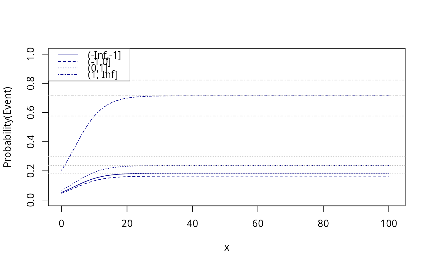
x <- seq(0,100,length.out=100)
newdata <- expand.grid(x=x,age=20,z=levels(d$z))
fit <- predict(e,newdata=newdata)
plot(0,0,type="n",xlim=c(0,101),ylim=c(0,1),xlab="x",ylab="Probability(Event)")
count <- 0
for (i in levels(newdata$z)) {
  count <- count+1
  lines(x,fit[which(newdata$z==i)],col="darkblue",lty=count)
}
abline(h=prev[3:4,1],lty=3:4,col="gray")
abline(h=prev[3:4,2],lty=3:4,col="lightgray")
abline(h=prev[3:4,3],lty=3:4,col="lightgray")
legend("topleft",levels(d$z),col="darkblue",lty=seq_len(length(levels(d$z))))