Model Fit for Survival Data

Model fit for survival data: the integrated Brier score for censored observations.

sbrier(obj, pred, btime= range(obj[,1]))

Arguments

obj: an object of class Surv.
pred: predicted values. Either a probability or a list of survfit objects.
btime: numeric vector of times, the integrated Brier score is computed if this is of length > 1. The Brier score at btime is returned otherwise.

Details

There is no obvious criterion of model fit for censored data. The Brier score for censoring as well as it's integrated version were suggested by Graf et al (1999).

The integrated Brier score is always computed over a subset of the interval given by the range of the time slot of the survival object obj.

Value

The (integrated) Brier score with attribute time is returned.

References

Erika Graf, Claudia Schmoor, Willi Sauerbrei and Martin Schumacher (1999), Assessment and comparison of prognostic classification schemes for survival data. Statistics in Medicine 18(17-18), 2529–2545.

Examples


library("survival")
data("DLBCL", package = "ipred")
smod <- Surv(DLBCL$time, DLBCL$cens)

KM <- survfit(smod ~ 1)
# integrated Brier score up to max(DLBCL$time)
sbrier(smod, KM)
#>           [,1]
#> [1,] 0.2237226
#> attr(,"names")
#> [1] "integrated Brier score"
#> attr(,"time")
#> [1]   1.3 129.9

# integrated Brier score up to time=50
sbrier(smod, KM, btime=c(0, 50))
#> Warning: btime[1] is smaller than min(time)
#>           [,1]
#> [1,] 0.2174081
#> attr(,"names")
#> [1] "integrated Brier score"
#> attr(,"time")
#> [1]  1.3 39.6

# Brier score for time=50
sbrier(smod, KM, btime=50)
#> Brier score 
#>    0.249375 
#> attr(,"time")
#> [1] 50

# a "real" model: one single survival tree with Intern. Prognostic Index
# and mean gene expression in the first cluster as predictors
mod <- bagging(Surv(time, cens) ~ MGEc.1 + IPI, data=DLBCL, nbagg=1)

# this is a list of survfit objects (==KM-curves), one for each observation
# in DLBCL
pred <- predict(mod, newdata=DLBCL)

# integrated Brier score up to max(time)
sbrier(smod, pred)
#>           [,1]
#> [1,] 0.1442559
#> attr(,"names")
#> [1] "integrated Brier score"
#> attr(,"time")
#> [1]   1.3 129.9

# Brier score at time=50
sbrier(smod, pred, btime=50)
#> Brier score 
#>   0.1774478 
#> attr(,"time")
#> [1] 50
# artificial examples and illustrations

cleans <- function(x) { attr(x, "time") <- NULL; names(x) <- NULL; x }

n <- 100
time <- rpois(n, 20)
cens <- rep(1, n)

# checks, Graf et al. page 2536, no censoring at all!
# no information: \pi(t) = 0.5 

a <- sbrier(Surv(time, cens), rep(0.5, n), time[50])
stopifnot(all.equal(cleans(a),0.25))

# some information: \pi(t) = S(t)

n <- 100
time <- 1:100
mod <- survfit(Surv(time, cens) ~ 1)
a <- sbrier(Surv(time, cens), rep(list(mod), n))
mymin <- mod$surv * (1 - mod$surv)
cleans(a)
#>           [,1]
#> [1,] 0.1682833
sum(mymin)/diff(range(time))
#> [1] 0.1683333

# independent of ordering
rand <- sample(1:100)
b <- sbrier(Surv(time, cens)[rand], rep(list(mod), n)[rand])
stopifnot(all.equal(cleans(a), cleans(b)))


# 2 groups at different risk

time <- c(1:10, 21:30)
strata <- c(rep(1, 10), rep(2, 10))
cens <- rep(1, length(time))

# no information about the groups

a <- sbrier(Surv(time, cens), survfit(Surv(time, cens) ~ 1))
b <- sbrier(Surv(time, cens), rep(list(survfit(Surv(time, cens) ~1)), 20))
stopifnot(all.equal(a, b))

# risk groups known

mod <- survfit(Surv(time, cens) ~ strata)
b <- sbrier(Surv(time, cens), c(rep(list(mod[1]), 10), rep(list(mod[2]), 10)))
stopifnot(a > b)

### GBSG2 data
data("GBSG2", package = "TH.data")

thsum <- function(x) {
  ret <- c(median(x), quantile(x, 0.25), quantile(x,0.75))
  names(ret)[1] <- "Median"
  ret
}

t(apply(GBSG2[,c("age", "tsize", "pnodes",
                 "progrec", "estrec")], 2, thsum))
#>         Median 25%    75%
#> age       53.0  46  61.00
#> tsize     25.0  20  35.00
#> pnodes     3.0   1   7.00
#> progrec   32.5   7 131.75
#> estrec    36.0   8 114.00

table(GBSG2$menostat)
#> 
#>  Pre Post 
#>  290  396 
table(GBSG2$tgrade)
#> 
#>   I  II III 
#>  81 444 161 
table(GBSG2$horTh)
#> 
#>  no yes 
#> 440 246 

# pooled Kaplan-Meier

mod <- survfit(Surv(time, cens) ~ 1, data=GBSG2)
# integrated Brier score
sbrier(Surv(GBSG2$time, GBSG2$cens), mod)
#>           [,1]
#> [1,] 0.1939366
#> attr(,"names")
#> [1] "integrated Brier score"
#> attr(,"time")
#> [1]    8 2659
# Brier score at 5 years
sbrier(Surv(GBSG2$time, GBSG2$cens), mod, btime=1825)
#> Brier score 
#>   0.2499984 
#> attr(,"time")
#> [1] 1825

# Nottingham prognostic index

GBSG2 <- GBSG2[order(GBSG2$time),]

NPI <- 0.2*GBSG2$tsize/10 + 1 + as.integer(GBSG2$tgrade)
NPI[NPI < 3.4] <- 1
NPI[NPI >= 3.4 & NPI <=5.4] <- 2
NPI[NPI > 5.4] <- 3

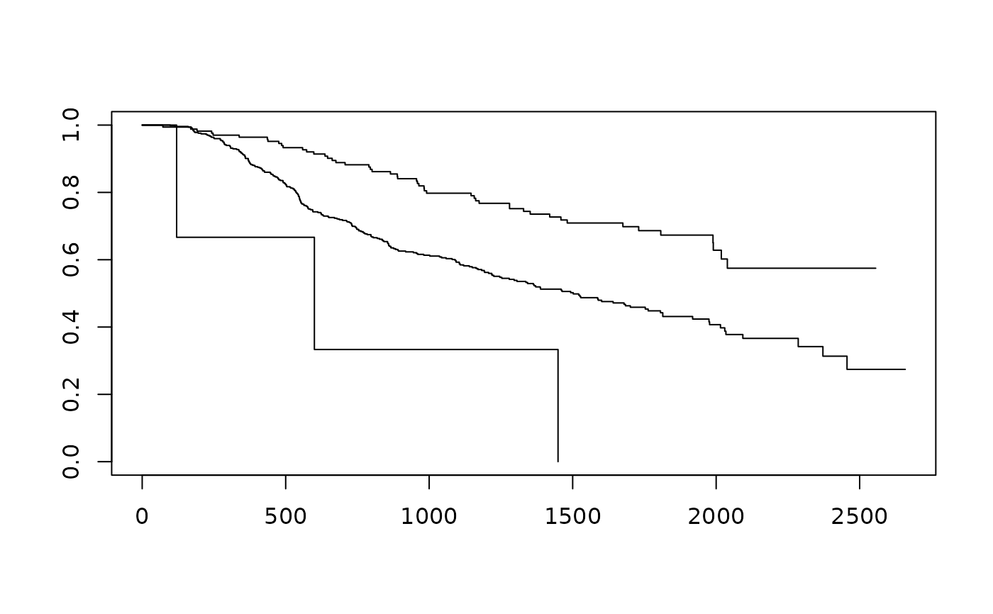
mod <- survfit(Surv(time, cens) ~ NPI, data=GBSG2)
plot(mod)


pred <- c()
survs <- c()
for (i in sort(unique(NPI)))
    survs <- c(survs, getsurv(mod[i], 1825))

for (i in 1:nrow(GBSG2))
   pred <- c(pred, survs[NPI[i]])

# Brier score of NPI at t=5 years
sbrier(Surv(GBSG2$time, GBSG2$cens), pred, btime=1825)
#> Brier score 
#>    0.233823 
#> attr(,"time")
#> [1] 1825

Arguments

Details

Value

See also

References

Examples