Bivariate Interpolation for Data on a Rectangular grid

This is a placeholder function for backward compatibility with packaga akima.

In its current state it simply calls the reimplemented Akima algorithm for irregular grids applied to the regular gridded data given.

Later a reimplementation of the original algorithm for regular grids may follow.

bicubic(x, y, z, x0, y0)

Arguments

x

a vector containing the x coordinates of the rectangular data grid.

y

a vector containing the y coordinates of the rectangular data grid.

z

a matrix containing the z[i,j] data values for the grid points (x[i],y[j]).

x0

vector of x coordinates used to interpolate at.

y0

vector of y coordinates used to interpolate at.

Details

This function is a call wrapper for backward compatibility with package akima.

Currently it applies Akimas irregular grid splines to regular grids, later a FOSS reimplementation of his regular grid splines may replace this wrapper.

Value

This function produces a list of interpolated points:

x

vector of x coordinates.

y

vector of y coordinates.

z

vector of interpolated data z.

If you need an output grid, see bicubic.grid.

References

Akima, H. (1996) Rectangular-Grid-Data Surface Fitting that Has the Accuracy of a Bicubic Polynomial, J. ACM 22(3), 357-361

Note

Use interp for the general case of irregular gridded data!

See also

interp, bicubic.grid

Examples

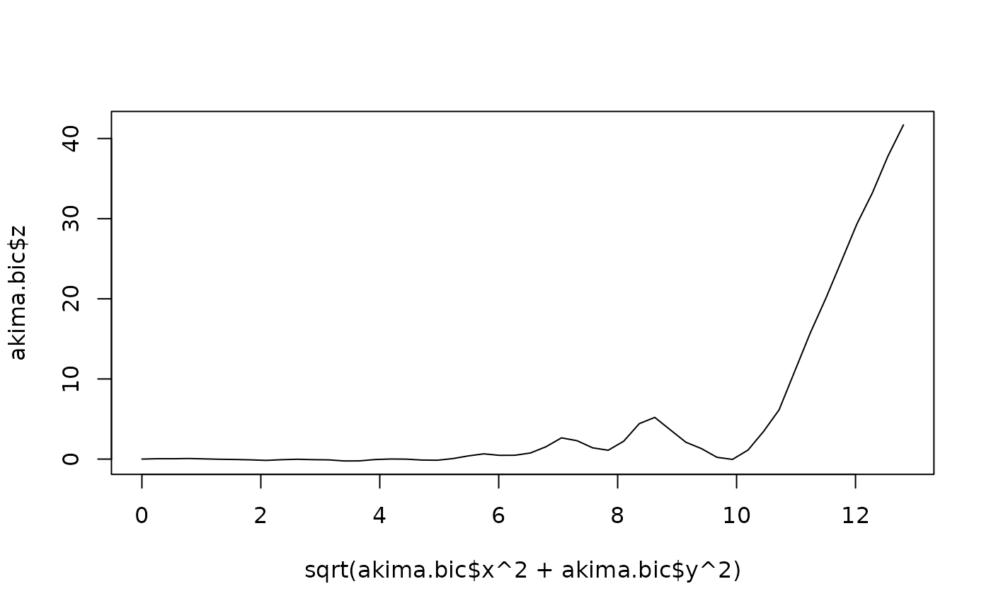
data(akima474)
# interpolate at the diagonal of the grid [0,8]x[0,10]
akima.bic <- bicubic(akima474$x,akima474$y,akima474$z,
                     seq(0,8,length=50), seq(0,10,length=50))
#> Warning: this output is generated according to Akimas irregular grid splines, not the regular grid one! This is a temporary workaround until Akimas ACM algorithm 760 is reimplmented from scratch!
plot(sqrt(akima.bic$x^2+akima.bic$y^2), akima.bic$z, type="l")