Hexagon Coordinates and Polygon Drawing
hexpolygon.RdSimple ‘low-level’ function for computing and drawing hexagons. Can be used for ‘grid’ (package grid) or ‘traditional’ (package graphics) graphics.
Usage
hexcoords(dx, dy = NULL, n = 1, sep = NULL)

hexpolygon(x, y, hexC = hexcoords(dx, dy, n = 1), dx, dy = NULL,
           fill = 1, border = 0, hUnit = "native", ...)
Arguments
- dx,dy
horizontal and vertical width of the hexagon(s).
- n
number of hexagon “repeats”.
- sep
separator value to be put between coordinates of different hexagons. The default,
NULLdoesn't use a separator.- x,y
numeric vectors of the same length specifying the hexagon centers around which to draw.
- hexC
a list as returned from
hexcoords(). Its componentno.sepdetermines if grid or traditional graphics are used. The default (via default ofhexcoords) is now to use grid graphics.- fill,border
passed to
grid.polygon(for grid).- hUnit
string or
NULLdetermining in which units (x,y) values are.- ...
further arguments passed to
polygon(for graphics).
Value
hexcoords() returns a list with components
- x,y
numeric vectors of length \(n \times 6\) (or \(n \times 7\) if
sepis not NULL) specifying the hexagon polygon coordinates (withsepappended to each 6-tuple).- no.sep
a logical indicating if
sepwasNULL.
hexpolygon returns what its last grid.polygon(.)
or polygon(.) call returns.
See also
grid.hexagons which builds on these.
Examples
str(hexcoords(1, sep = NA)) # multiple of (6 + 1)
#> List of 3
#> $ x : num [1:7] 1 1 0 -1 -1 0 NA
#> $ y : num [1:7] 0.577 -0.577 -1.155 -0.577 0.577 ...
#> $ no.sep: logi FALSE
str(hexcoords(1, sep = NULL))# no separator -> multiple of 6
#> List of 3
#> $ x : num [1:6] 1 1 0 -1 -1 0
#> $ y : num [1:6] 0.577 -0.577 -1.155 -0.577 0.577 ...
#> $ no.sep: logi TRUE
## hexpolygon()s:
x <- runif(20, -2, 2)
y <- x + rnorm(20)
## 1) traditional 'graphics'
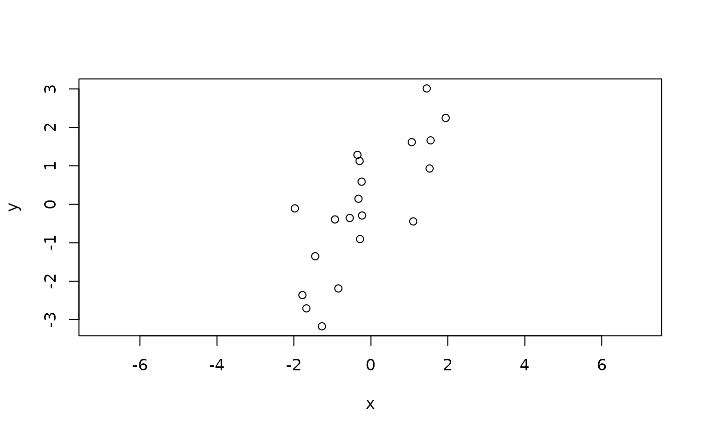
plot(x,y, asp = 1, "plot() + hexpolygon()")
#> Warning: plot type 'plot() + hexpolygon()' will be truncated to first character
hexpolygon(x,y, dx = 0.1, density = 25, col = 2, lwd = 1.5)
 ## 2) "grid" :
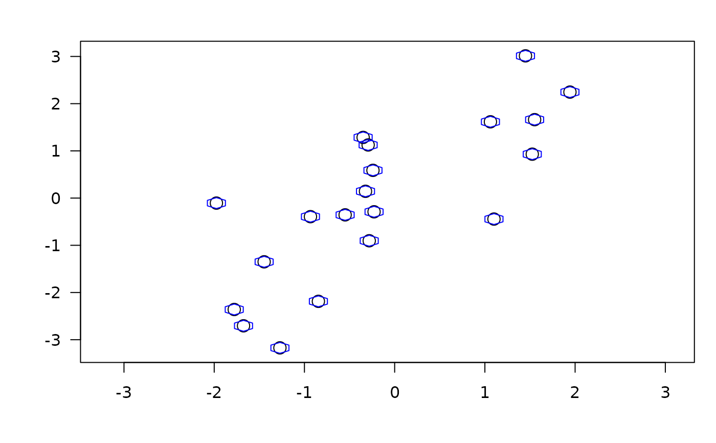
addBit <- function(bnds, f = 0.05) bnds + c(-f, f) * diff(bnds)
sc <- addBit(rxy <- range(x,y))# same extents (cheating asp=1)
library("grid")
grid.newpage()
pushViewport(plotViewport(.1+c(4,4,2,1), xscale = sc, yscale = sc))
grid.rect()
grid.xaxis()
grid.yaxis()
grid.points(x,y)
hexpolygon(x,y, hexcoords(dx = 0.1, sep=NULL), border = "blue", fill=NA)
popViewport()
## 2) "grid" :
addBit <- function(bnds, f = 0.05) bnds + c(-f, f) * diff(bnds)
sc <- addBit(rxy <- range(x,y))# same extents (cheating asp=1)
library("grid")
grid.newpage()
pushViewport(plotViewport(.1+c(4,4,2,1), xscale = sc, yscale = sc))
grid.rect()
grid.xaxis()
grid.yaxis()
grid.points(x,y)
hexpolygon(x,y, hexcoords(dx = 0.1, sep=NULL), border = "blue", fill=NA)
popViewport()