Add Regression Line Equation and R-Square to a GGPLOT.

Add regression line equation and R^2 to a ggplot. Regression model is fitted using the function lm.

Usage

stat_regline_equation(
  mapping = NULL,
  data = NULL,
  formula = y ~ x,
  label.x.npc = "left",
  label.y.npc = "top",
  label.x = NULL,
  label.y = NULL,
  output.type = "expression",
  decreasing = TRUE,
  geom = "text",
  position = "identity",
  na.rm = FALSE,
  show.legend = NA,
  inherit.aes = TRUE,
  ...
)

Arguments

mapping

Set of aesthetic mappings created by aes(). If specified and inherit.aes = TRUE (the default), it is combined with the default mapping at the top level of the plot. You must supply mapping if there is no plot mapping.

data

The data to be displayed in this layer. There are three options:

If NULL, the default, the data is inherited from the plot data as specified in the call to ggplot().

A data.frame, or other object, will override the plot data. All objects will be fortified to produce a data frame. See fortify() for which variables will be created.

A function will be called with a single argument, the plot data. The return value must be a data.frame, and will be used as the layer data. A function can be created from a formula (e.g. ~ head(.x, 10)).

formula

a formula object

label.x.npc, label.y.npc

can be numeric or character vector of the same length as the number of groups and/or panels. If too short they will be recycled.

If numeric, value should be between 0 and 1. Coordinates to be used for positioning the label, expressed in "normalized parent coordinates".
If character, allowed values include: i) one of c('right', 'left', 'center', 'centre', 'middle') for x-axis; ii) and one of c( 'bottom', 'top', 'center', 'centre', 'middle') for y-axis.

If too short they will be recycled.

label.x, label.y

numeric Coordinates (in data units) to be used for absolute positioning of the label. If too short they will be recycled.

output.type

character One of "expression", "latex" or "text".

decreasing

logical. If TRUE (the default), the equation is formatted in standard mathematical convention with terms in decreasing order of powers (e.g., "y = 2*x + 1"). If FALSE, terms are in increasing order (e.g., "y = 1 + 2*x").

geom

The geometric object to use to display the data for this layer. When using a stat_*() function to construct a layer, the geom argument can be used to override the default coupling between stats and geoms. The geom argument accepts the following:

A Geom ggproto subclass, for example GeomPoint.
A string naming the geom. To give the geom as a string, strip the function name of the geom_ prefix. For example, to use geom_point(), give the geom as "point".
For more information and other ways to specify the geom, see the layer geom documentation.

position

A position adjustment to use on the data for this layer. This can be used in various ways, including to prevent overplotting and improving the display. The position argument accepts the following:

The result of calling a position function, such as position_jitter(). This method allows for passing extra arguments to the position.
A string naming the position adjustment. To give the position as a string, strip the function name of the position_ prefix. For example, to use position_jitter(), give the position as "jitter".
For more information and other ways to specify the position, see the layer position documentation.

na.rm

If FALSE (the default), removes missing values with a warning. If TRUE silently removes missing values.

show.legend

logical. Should this layer be included in the legends? NA, the default, includes if any aesthetics are mapped. FALSE never includes, and TRUE always includes. It can also be a named logical vector to finely select the aesthetics to display. To include legend keys for all levels, even when no data exists, use TRUE. If NA, all levels are shown in legend, but unobserved levels are omitted.

inherit.aes

If FALSE (the default for most ggpubr functions), overrides the default aesthetics, rather than combining with them. This is most useful for helper functions that define both data and aesthetics and shouldn't inherit behaviour from the default plot specification. Set to TRUE to inherit aesthetics from the parent ggplot layer.

...

other arguments to pass to geom_text or geom_label.

Computed variables

x: x position for left edge
y: y position near upper edge
eq.label: equation for the fitted polynomial as a character string to be parsed
rr.label: \(R^2\) of the fitted model as a character string to be parsed
adj.rr.label: Adjusted \(R^2\) of the fitted model as a character string to be parsed
AIC.label: AIC for the fitted model.
BIC.label: BIC for the fitted model.
hjust: Set to zero to override the default of the "text" geom.

References

the source code of the function stat_regline_equation() is inspired from the code of the function stat_poly_eq() (in ggpmisc package).

Examples


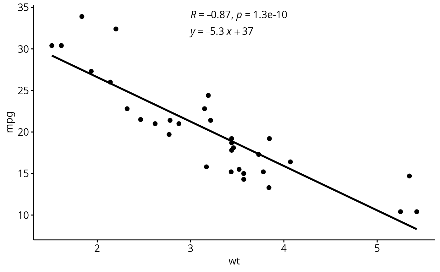
# Simple scatter plot with correlation coefficient and
# regression line
#::::::::::::::::::::::::::::::::::::::::::::::::::::
ggscatter(mtcars, x = "wt", y = "mpg", add = "reg.line") +
  stat_cor(label.x = 3, label.y = 34) +
  stat_regline_equation(label.x = 3, label.y = 32)



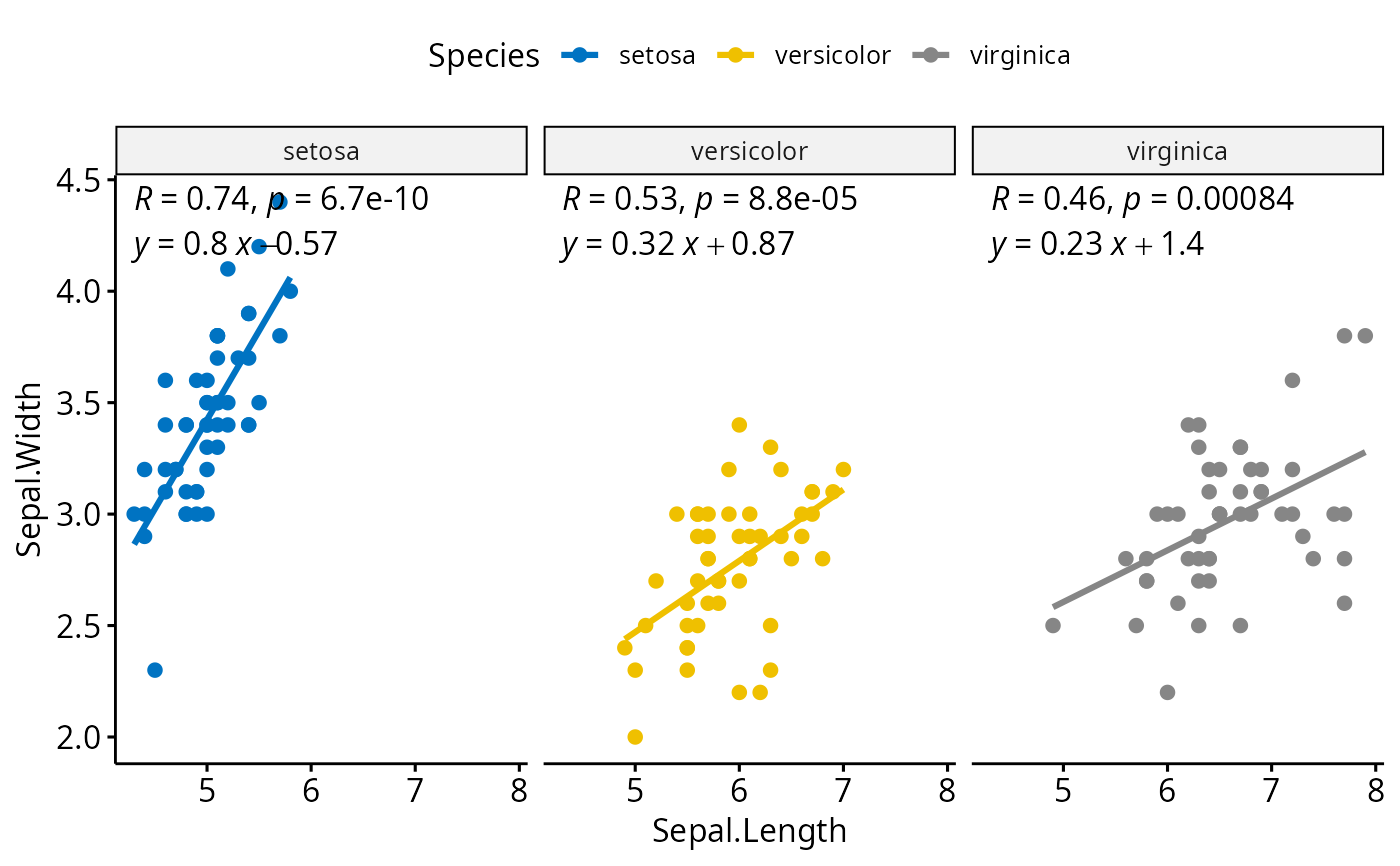
# Groupped scatter plot
#::::::::::::::::::::::::::::::::::::::::::::::::::::
ggscatter(
  iris, x = "Sepal.Length", y = "Sepal.Width",
  color = "Species", palette = "jco",
  add = "reg.line"
  ) +
  facet_wrap(~Species) +
  stat_cor(label.y = 4.4) +
  stat_regline_equation(label.y = 4.2)


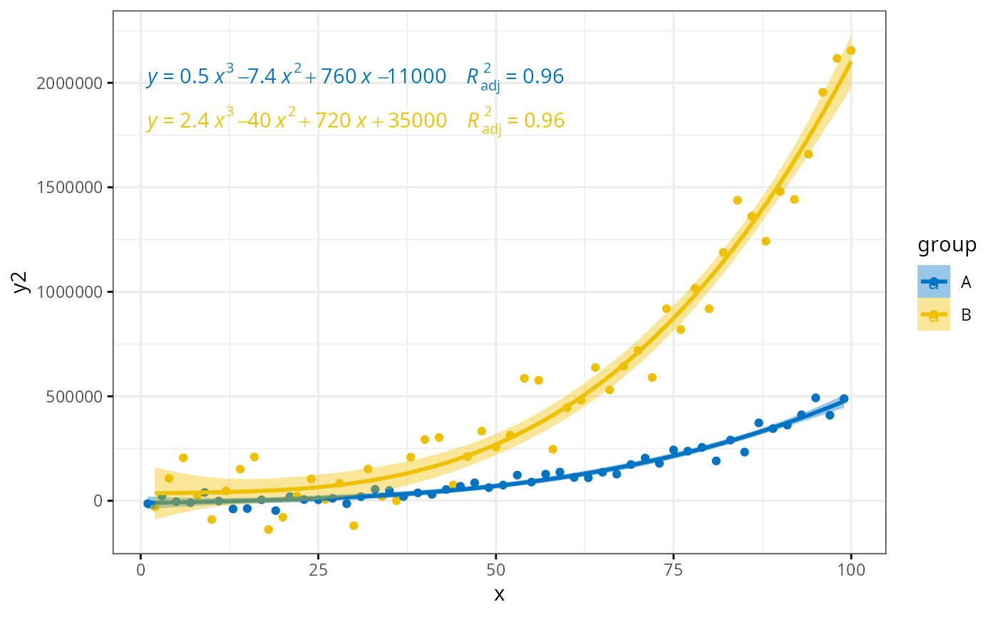
# Polynomial equation
#::::::::::::::::::::::::::::::::::::::::::::::::::::

# Demo data
set.seed(4321)
x <- 1:100
y <- (x + x^2 + x^3) + rnorm(length(x), mean = 0, sd = mean(x^3) / 4)
my.data <- data.frame(x, y, group = c("A", "B"),
                      y2 = y * c(0.5,2), block = c("a", "a", "b", "b"))

# Fit polynomial regression line and add labels
formula <- y ~ poly(x, 3, raw = TRUE)
p <- ggplot(my.data, aes(x, y2, color = group)) +
  geom_point() +
  stat_smooth(aes(fill = group, color = group), method = "lm", formula = formula) +
  stat_regline_equation(
    aes(label =  paste(..eq.label.., ..adj.rr.label.., sep = "~~~~")),
    formula = formula
  ) +
  theme_bw()
ggpar(p, palette = "jco")

Usage

Arguments

Computed variables

References

See also

Examples