Monotone Regression: Isotonic Regression and Antitonic Regression

monoreg performs monotone regression (either isotonic or antitonic) with weights.

monoreg(x, y=NULL, w=rep(1, length(x)), type=c("isotonic", "antitonic"))

Arguments

x, y: coordinate vectors of the regression points. Alternatively a single “plotting” structure can be specified: see xy.coords.
w: data weights (default values: 1).
type: fit a monotonely increasing ("isotonic") or monotonely decreasing ("antitonic") function.

Details

monoreg is similar to isoreg, with the addition that monoreg accepts weights.

If several identical x values are given as input, the corresponding y values and the weights w are automatically merged, and a warning is issued.

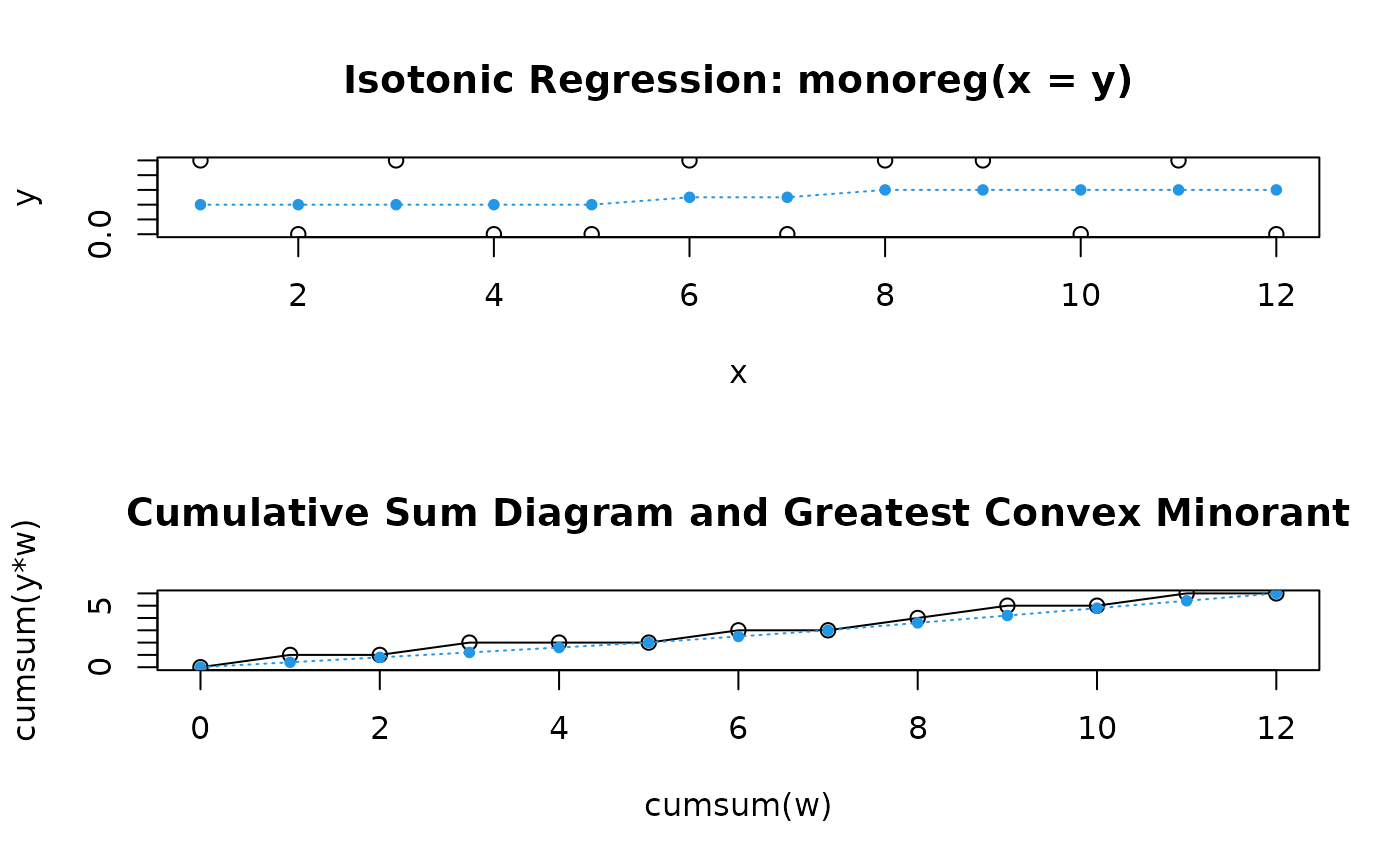
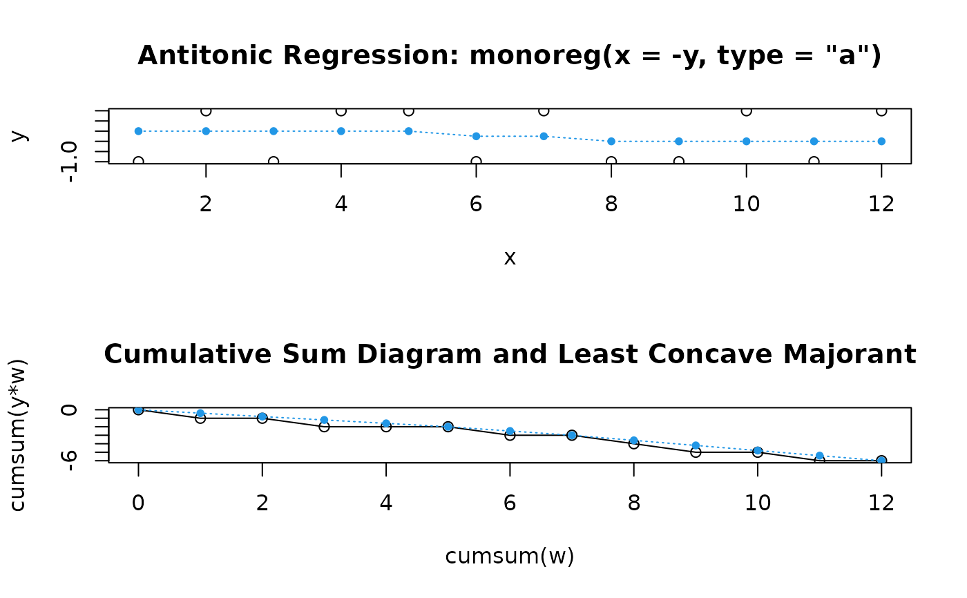
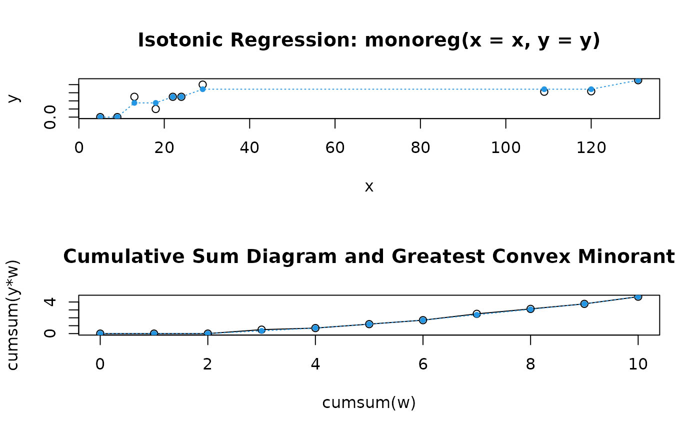
The plot.monoreg function optionally plots the cumulative sum diagram with the greatest convex minorant (isotonic regression) or the least concave majorant (antitonic regression), see the examples below.

Value

A list with the following entries:

x: the sorted and unique x values
y: the corresponding y values
w: the corresponding weights
yf: the fitted y values
type: the type of monotone regression ("isotonic" or "antitonic"
call: the function call

References

Robertson, T., F. T. Wright, and R. L. Dykstra. 1988. Order restricted statistical inference. John Wiley and Sons.

Author

Korbinian Strimmer (https://strimmerlab.github.io).

Part of this function is C code that has been ported from R code originally written by Kaspar Rufibach.

Examples

# load "fdrtool" library
library("fdrtool")


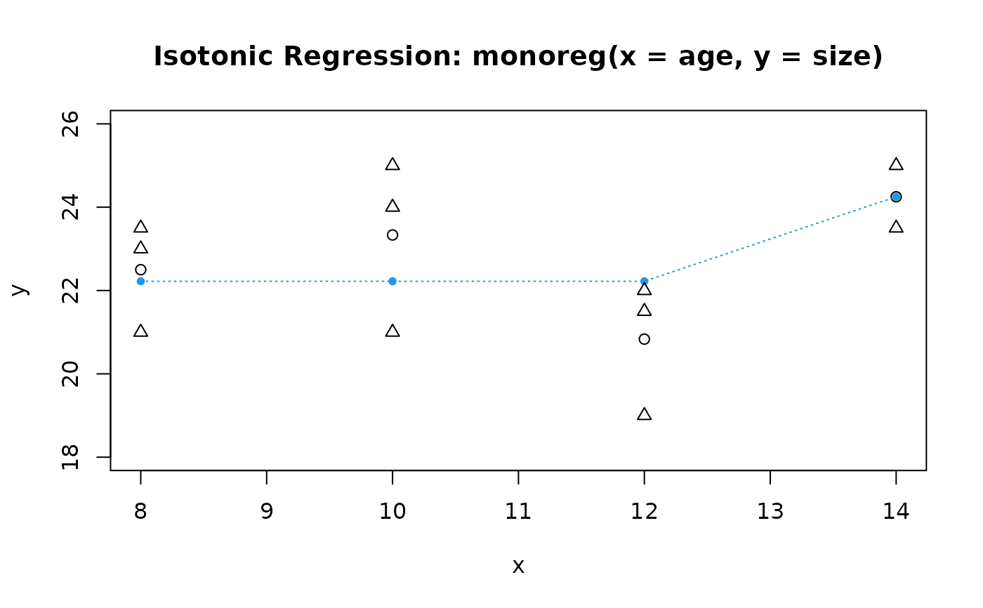
# an example with weights

# Example 1.1.1. (dental study) from Robertson, Wright and Dykstra (1988)
age = c(14, 14, 8, 8, 8, 10, 10, 10, 12, 12, 12)
size = c(23.5, 25, 21, 23.5, 23, 24, 21, 25, 21.5, 22, 19)

mr = monoreg(age, size)
#> Warning: Duplicated x value (x=14) detected!
#> The corresponding weights and y values will be merged.
#> Warning: Duplicated x value (x=8) detected!
#> The corresponding weights and y values will be merged.
#> Warning: Duplicated x value (x=10) detected!
#> The corresponding weights and y values will be merged.
#> Warning: Duplicated x value (x=12) detected!
#> The corresponding weights and y values will be merged.

# sorted x values
mr$x # 8 10 12 14
#> [1]  8 10 12 14
# weights and merged y values
mr$w  # 3 3 3 2
#> [1] 3 3 3 2
mr$y #  22.50000 23.33333 20.83333 24.25000
#> [1] 22.50000 23.33333 20.83333 24.25000
# fitted y values
mr$yf # 22.22222 22.22222 22.22222 24.25000
#> [1] 22.22222 22.22222 22.22222 24.25000
fitted(mr)
#> [1] 22.22222 22.22222 22.22222 24.25000
residuals(mr)
#> [1]  0.2777778  1.1111111 -1.3888889  0.0000000

plot(mr, ylim=c(18, 26))  # this shows the averaged data points
points(age, size, pch=2)  # add original data points



###

y = c(1,0,1,0,0,1,0,1,1,0,1,0)
x = 1:length(y)
mr = monoreg(y)

# plot with greatest convex minorant
plot(mr, plot.type="row.wise")  


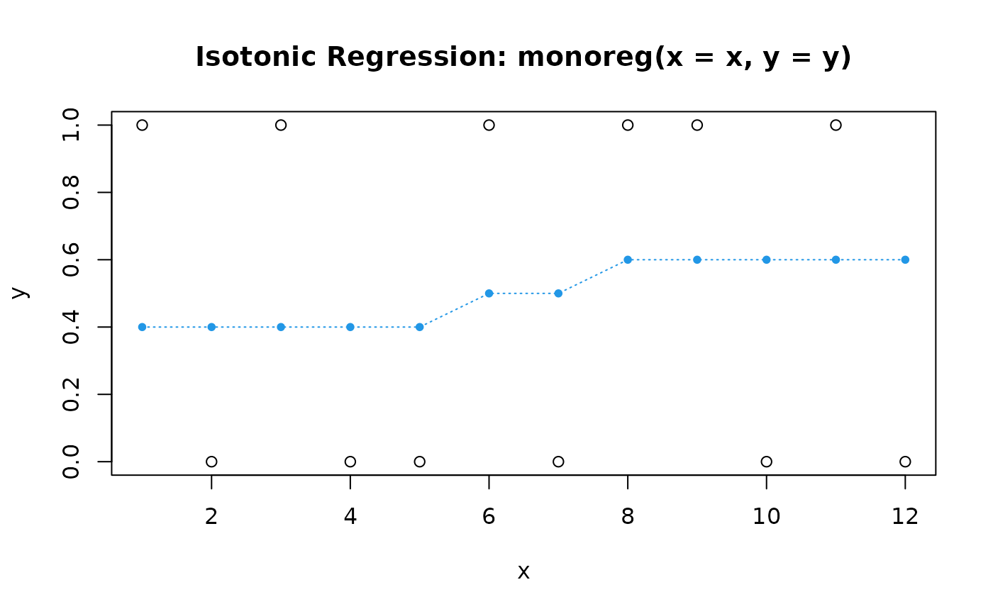
# this is the same
mr = monoreg(x,y)
plot(mr)


# antitonic regression and least concave majorant
mr = monoreg(-y, type="a")
plot(mr, plot.type="row.wise")  


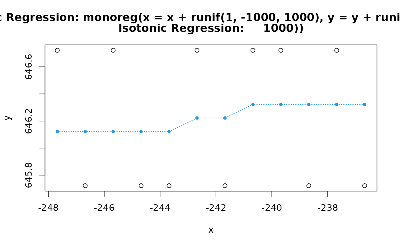
# the fit yf is independent of the location of x and y
plot(monoreg(x + runif(1, -1000, 1000), 
             y +runif(1, -1000, 1000)) )


###

y = c(0,0,2/4,1/5,2/4,1/2,4/5,5/8,7/11,10/11)
x = c(5,9,13,18,22,24,29,109,120,131)

mr = monoreg(x,y)
plot(mr, plot.type="row.wise")


# the fit (yf) only depends on the ordering of x
monoreg(1:length(y), y)$yf 
#>  [1] 0.0000000 0.0000000 0.3500000 0.3500000 0.5000000 0.5000000 0.6871212
#>  [8] 0.6871212 0.6871212 0.9090909
monoreg(x, y)$yf 
#>  [1] 0.0000000 0.0000000 0.3500000 0.3500000 0.5000000 0.5000000 0.6871212
#>  [8] 0.6871212 0.6871212 0.9090909