The Half-Normal Distribution
halfnorm.RdDensity, distribution function, quantile function and random
generation for the half-normal distribution with parameter theta.
Arguments
- x,q
vector of quantiles.
- p
vector of probabilities.
- n
number of observations. If
length(n) > 1, the length is taken to be the number required.- theta
parameter of half-normal distribution.
- log, log.p
logical; if TRUE, probabilities p are given as log(p).
- lower.tail
logical; if TRUE (default), probabilities are \(P[X \le x]\), otherwise, \(P[X > x]\).
- sd
standard deviation of the zero-mean normal distribution that corresponds to the half-normal with parameter
theta.
Value
dhalfnorm gives the density,
phalfnorm gives the distribution function,
qhalfnorm gives the quantile function, and
rhalfnorm generates random deviates.
sd2theta computes a theta parameter.
theta2sd computes a sd parameter.
Details
x = abs(z) follows a half-normal distribution with
if z is a normal variate with zero mean.
The half-normal distribution has density
$$
f(x) =
\frac{2 \theta}{\pi} e^{-x^2 \theta^2/\pi}$$
It has mean \(E(x) = \frac{1}{\theta}\) and variance
\(Var(x) = \frac{\pi-2}{2 \theta^2}\).
The parameter \(\theta\) is related to the standard deviation \(\sigma\) of the corresponding zero-mean normal distribution by the equation \(\theta = \sqrt{\pi/2}/\sigma\).
If \(\theta\) is not specified in the above functions it assumes the default values of \(\sqrt{\pi/2}\), corresponding to \(\sigma=1\).
See also
Examples
# load "fdrtool" library
library("fdrtool")
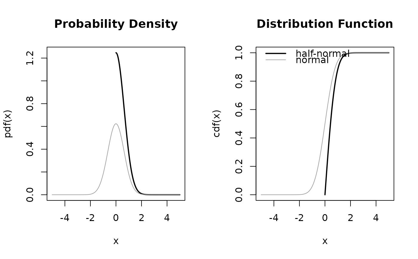
## density of half-normal compared with a corresponding normal
par(mfrow=c(1,2))
sd.norm = 0.64
x = seq(0, 5, 0.01)
x2 = seq(-5, 5, 0.01)
plot(x, dhalfnorm(x, sd2theta(sd.norm)), type="l", xlim=c(-5, 5), lwd=2,
main="Probability Density", ylab="pdf(x)")
lines(x2, dnorm(x2, sd=sd.norm), col=8 )
plot(x, phalfnorm(x, sd2theta(sd.norm)), type="l", xlim=c(-5, 5), lwd=2,
main="Distribution Function", ylab="cdf(x)")
lines(x2, pnorm(x2, sd=sd.norm), col=8 )
legend("topleft",
c("half-normal", "normal"), lwd=c(2,1),
col=c(1, 8), bty="n", cex=1.0)
 par(mfrow=c(1,1))
## distribution function
integrate(dhalfnorm, 0, 1.4, theta = 1.234)
#> 0.831928 with absolute error < 9.2e-15
phalfnorm(1.4, theta = 1.234)
#> [1] 0.831928
## quantile function
qhalfnorm(-1) # NaN
#> [1] NaN
qhalfnorm(0)
#> [1] 0
qhalfnorm(.5)
#> [1] 0.6744898
qhalfnorm(1)
#> [1] Inf
qhalfnorm(2) # NaN
#> Warning: NaNs produced
#> [1] NaN
## random numbers
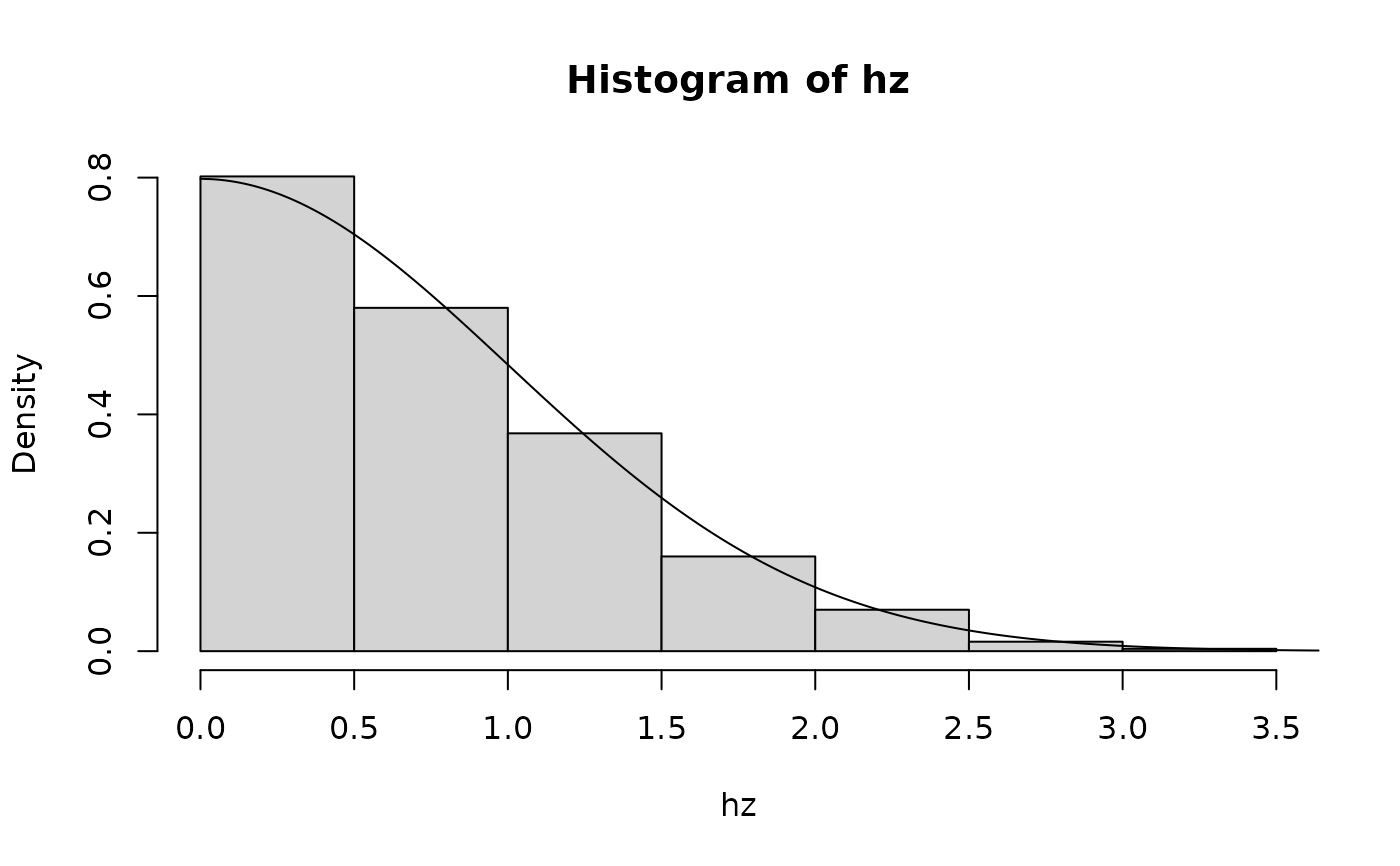
theta = 0.72
hz = rhalfnorm(10000, theta)
hist(hz, freq=FALSE)
lines(x, dhalfnorm(x, theta))
par(mfrow=c(1,1))
## distribution function
integrate(dhalfnorm, 0, 1.4, theta = 1.234)
#> 0.831928 with absolute error < 9.2e-15
phalfnorm(1.4, theta = 1.234)
#> [1] 0.831928
## quantile function
qhalfnorm(-1) # NaN
#> [1] NaN
qhalfnorm(0)
#> [1] 0
qhalfnorm(.5)
#> [1] 0.6744898
qhalfnorm(1)
#> [1] Inf
qhalfnorm(2) # NaN
#> Warning: NaNs produced
#> [1] NaN
## random numbers
theta = 0.72
hz = rhalfnorm(10000, theta)
hist(hz, freq=FALSE)
lines(x, dhalfnorm(x, theta))
 mean(hz)
#> [1] 1.380705
1/theta # theoretical mean
#> [1] 1.388889
var(hz)
#> [1] 1.10687
(pi-2)/(2*theta*theta) # theoretical variance
#> [1] 1.101073
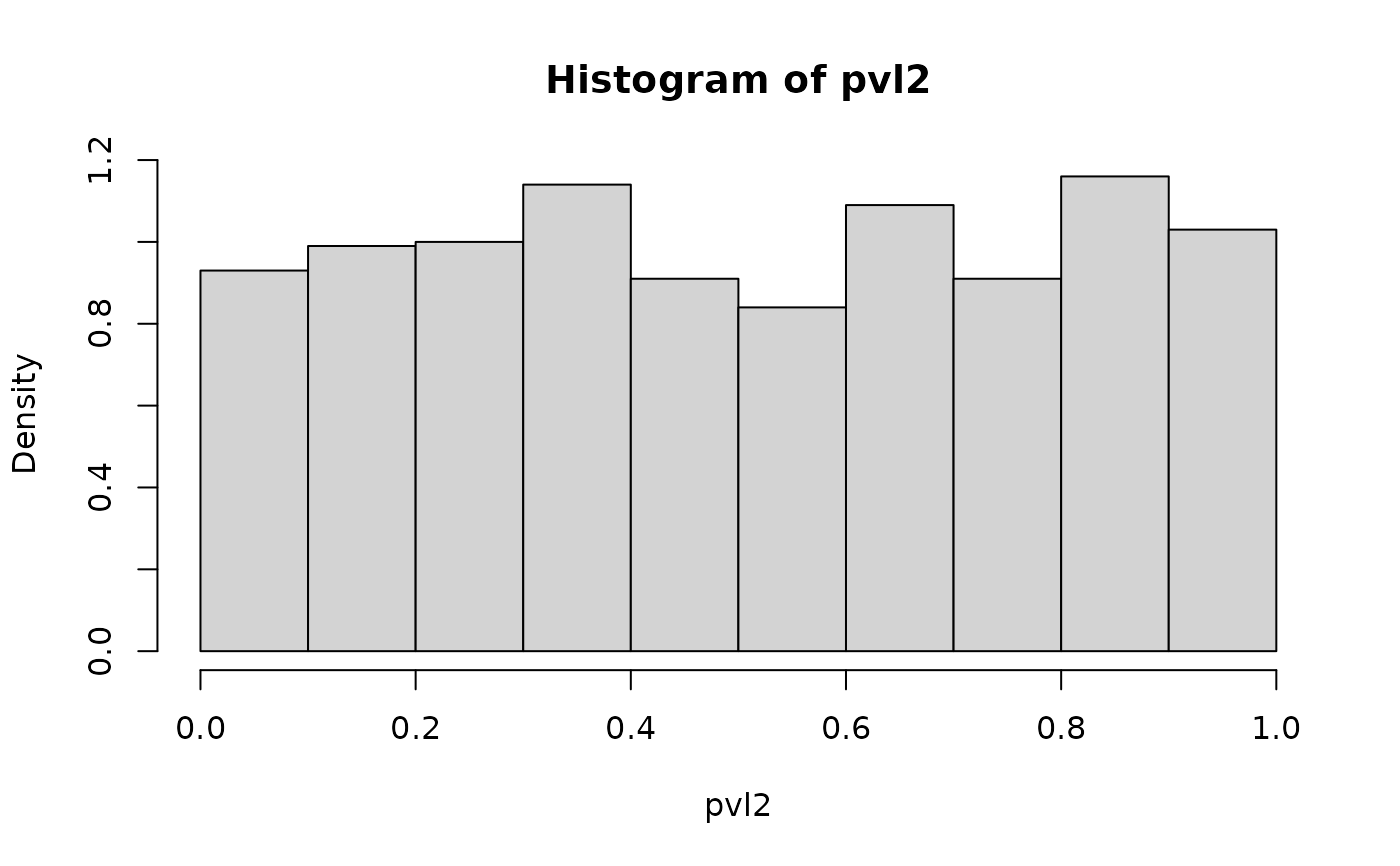
## relationship with two-sided normal p-values
z = rnorm(1000)
# two-sided p-values
pvl = 1- phalfnorm(abs(z))
pvl2 = 2 - 2*pnorm(abs(z))
sum(pvl-pvl2)^2 # equivalent
#> [1] 0
hist(pvl2, freq=FALSE) # uniform distribution
mean(hz)
#> [1] 1.380705
1/theta # theoretical mean
#> [1] 1.388889
var(hz)
#> [1] 1.10687
(pi-2)/(2*theta*theta) # theoretical variance
#> [1] 1.101073
## relationship with two-sided normal p-values
z = rnorm(1000)
# two-sided p-values
pvl = 1- phalfnorm(abs(z))
pvl2 = 2 - 2*pnorm(abs(z))
sum(pvl-pvl2)^2 # equivalent
#> [1] 0
hist(pvl2, freq=FALSE) # uniform distribution
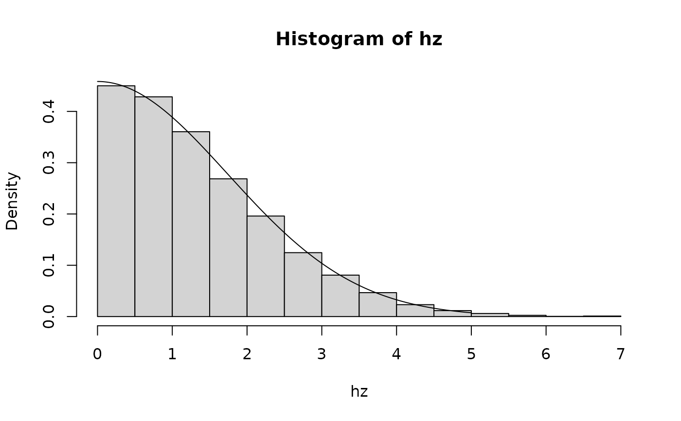
 # back to half-normal scores
hz = qhalfnorm(1-pvl)
hist(hz, freq=FALSE)
lines(x, dhalfnorm(x))
# back to half-normal scores
hz = qhalfnorm(1-pvl)
hist(hz, freq=FALSE)
lines(x, dhalfnorm(x))