Distribution of One and Two Sample Permutation Tests

Density, distribution function and quantile function for the distribution of one and two sample permutation tests using the Shift-Algorithm by Streitberg & R\"ohmel.

Usage

dperm(x, scores, m, paired=NULL, tol = 0.01, fact=NULL, density=FALSE,
      simulate=FALSE, B=10000)
pperm(q, scores, m, paired=NULL, tol = 0.01, fact=NULL,
      alternative=c("less", "greater", "two.sided"), pprob=FALSE,
      simulate=FALSE, B=10000)
qperm(p, scores, m, paired=NULL, tol = 0.01, fact=NULL, 
      simulate=FALSE, B=10000)
rperm(n, scores, m)

Arguments

x, q: vector of quantiles.
p: vector of probabilities.
scores: arbitrary scores of the observations of the x (first m elements) and y sample.
m: sample size of the x sample. If m = length(x) scores of paired observations are assumed.
paired: logical. Indicates if paired observations are used. Needed to discriminate between a paired problem and the distribution of the total sum of the scores (which has mass 1 at the point sum(scores)).

tol: real. Real valued scores are mapped into integers by rounding after multiplication with an appropriate factor. Make sure that the absolute difference between the each possible test statistic for the original scores and the rounded scores is less than tol. This might not be possible due to memory/time limitations, a warning is given in this case.
fact: real. If fact is given, real valued scores are mapped into integers using fact as factor. tol is ignored in this case.
n: number of random observations to generate.
alternative: character indicating whether the probability $P(T \le q)$ (less), $P(T \ge q)$ (greater) or a two-sided p-value (two.sided) should be computed in pperm.
pprob: logical. Indicates if the probability $P(T = q)$ should be computed additionally.
density: logical. When x is a scalar and density is TRUE, dperm returns the density for all possible statistics less or equal x as a data frame.
simulate: logical. Use conditional Monte-Carlo to compute the distribution.
B: number of Monte-Carlo replications to be used.

Details

The exact distribution of the sum of the first m scores is evaluated using the Shift-Algorithm by Streitberg & R\"ohmel under the hypothesis of exchangeability (or, equivalent, the hypothesis that all permutations of the scores are equally likely). The algorithm is able to deal with tied scores, so the conditional distribution can be evaluated.

The algorithm is defined for positive integer valued scores only. There are two ways dealing with real valued scores. First, one can try to find integer valued scores that lead to statistics which differ not more than tol from the statistics computed for the original scores. This can be done as follows.

Without loss of generality let $a_i > 0$ denote real valued scores in reverse ordering and $f$ a positive factor (this is the fact argument). Let $R_i = f \cdot a_i - round(f \cdot a_i)$. Then

$$ \sum_{i=1}^m f \cdot a_i = \sum_{i=1}^m round(f \cdot a_i) - R_i. $$

Clearly, the maximum difference between $1/f \sum_{i=1}^m f \cdot a_i$ and $1/f \sum_{i=1}^n round(f \cdot a_i)$ is given by $|\sum_{i=1}^m R_i|$. Therefore one searches for $f$ with

$$ |\sum_{i=1}^m R_i| \le \sum_{i=1}^m |R_i| \le tol.$$

If $f$ induces more that 100.000 columns in the Shift-Algorithm by Streitberg & R\"ohmel, $f$ is restricted to the largest integer that does not.

The second idea is to map the scores into integers by taking the integer part of $a_i N / \max(a_i)$ (Hothorn & Lausen, 2002). This induces additional ties, but the shape of the scores is very similar. That means we do not try to approximate something but use a different test (with integer valued scores), serving for the same purpose (due to a similar shape of the scores). However, this has to be done prior to calling pperm (see the examples).

Exact two-sided p-values are computed as suggested in the StatXact-5 manual, page 225, equation (9.31) and equation (8.18), p. 179 (paired case). In detail: For the paired case the two-sided p-value is just twice the one-sided one. For the independent sample case the two sided p-value is defined as $$p_2 = P( |T - E(T)| \ge | q - E(T) |)$$ where $q$ is the quantile passed to pperm.

Value

dperm gives the density, pperm gives the distribution function and qperm gives the quantile function. If pprob is true, pperm returns a list with elements

PVALUE: the probability specified by alternative.
PPROB: the probability $P(T = q)$.

rperm is a wrapper to sample.

References

Bernd Streitberg & Joachim R\"ohmel (1986), Exact distributions for permutations and rank tests: An introduction to some recently published algorithms. Statistical Software Newsletter 12(1), 10–17.

Bernd Streitberg & Joachim R\"ohmel (1987), Exakte Verteilungen f\"ur Rang- und Randomisierungstests im allgemeinen $c$-Stichprobenfall. EDV in Medizin und Biologie 18(1), 12–19.

Torsten Hothorn (2001), On exact rank tests in R. R News 1(1), 11–12.

Cyrus R. Mehta & Nitin R. Patel (2001), StatXact-5 for Windows. Manual, Cytel Software Cooperation, Cambridge, USA

Torsten Hothorn & Berthold Lausen (2003), On the exact distribution of maximally selected rank statistics. Computational Statistics & Data Analysis, 43(2), 121-137.

Examples


# exact one-sided p-value of the Wilcoxon test for a tied sample

x <- c(0.5, 0.5, 0.6, 0.6, 0.7, 0.8, 0.9)
y <- c(0.5, 1.0, 1.2, 1.2, 1.4, 1.5, 1.9, 2.0)
r <- cscores(c(x,y), type="Wilcoxon")
pperm(sum(r[seq(along=x)]), r, 7)
#> [1] 0.004351204

# Compare the exact algorithm as implemented in ctest and the
# Shift-Algorithm by Streitberg & Roehmel for untied samples
 
# Wilcoxon:

n <- 10
x <- rnorm(n, 2)
y <- rnorm(n, 3)
r <- cscores(c(x,y), type="Wilcoxon")

# exact distribution using the Shift-Algorithm

dwexac <- dperm((n*(n+1)/2):(n^2 + n*(n+1)/2), r, n)
sum(dwexac)           # should be something near 1 :-)
#> [1] 1

# exact distribution using dwilcox

dw <- dwilcox(0:(n^2), n, n)

# compare the two distributions:

plot(dw, dwexac, main="Wilcoxon", xlab="dwilcox", ylab="dperm")      

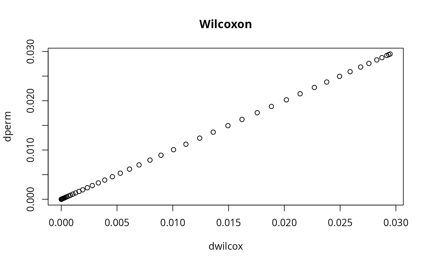# should give a "perfect" line

# Wilcoxon signed rank test

n <- 10
x <- rnorm(n, 5)
y <- rnorm(n, 5)
r <- cscores(abs(x - y), type="Wilcoxon")
pperm(sum(r[x - y > 0]), r, length(r))
#> [1] 0.7216797
wilcox.test(x,y, paired=TRUE, alternative="less")
#> 
#> 	Wilcoxon signed rank exact test
#> 
#> data:  x and y
#> V = 33, p-value = 0.7217
#> alternative hypothesis: true location shift is less than 0
#> 
psignrank(sum(r[x - y > 0]), length(r))
#> [1] 0.7216797

# Ansari-Bradley

n <- 10
x <- rnorm(n, 2, 1)
y <- rnorm(n, 2, 2)

# exact distribution using the Shift-Algorithm

sc <- cscores(c(x,y), type="Ansari")
dabexac <- dperm(0:(n*(2*n+1)/2), sc, n)
sum(dabexac)
#> [1] 1

# real scores are allowed (but only result in an approximation)
# e.g. v.d. Waerden test

n <- 10
x <- rnorm(n)
y <- rnorm(n)
scores <- cscores(c(x,y), type="NormalQuantile")
X <- sum(scores[seq(along=x)])  # <- v.d. Waerden normal quantile statistic

# critical value, two-sided test

abs(qperm(0.025, scores, length(x)))
#> Warning: cannot hold tol, tolerance: 0.010292
#> [1] 3.871345

# p-values

p1 <- pperm(X, scores, length(x), alternative="two.sided")
#> Warning: cannot hold tol, tolerance: 0.010292

# generate integer valued scores with the same shape as normal quantile
# scores, this no longer v.d.Waerden, but something very similar

scores <- cscores(c(x,y), type="NormalQuantile", int=TRUE)

X <- sum(scores[seq(along=x)])
p2 <- pperm(X, scores, length(x), alternative="two.sided")

# compare p1 and p2

p1 - p2
#> [1] -0.02262443