Discretize Continuous Random Variables

discretize puts observations from a continuous random variable into bins and returns the corresponding vector of counts.

discretize2d puts observations from a pair of continuous random variables into bins and returns the corresponding table of counts.

discretize( x, numBins, r=range(x) )
discretize2d( x1, x2, numBins1, numBins2, r1=range(x1), r2=range(x2) )

Arguments

x: vector of observations.
x1: vector of observations for the first random variable.
x2: vector of observations for the second random variable.
numBins: number of bins.
numBins1: number of bins for the first random variable.
numBins2: number of bins for the second random variable.
r: range of the random variable (default: observed range).
r1: range of the first random variable (default: observed range).
r2: range of the second random variable (default: observed range).

Details

The bins for a random variable all have the same width. It is determined by the length of the range divided by the number of bins.

Value

discretize returns a vector containing the counts for each bin.

discretize2d returns a matrix containing the counts for each bin.

Author

Korbinian Strimmer (https://strimmerlab.github.io).

Examples

# load entropy library 
library("entropy")

### 1D example ####

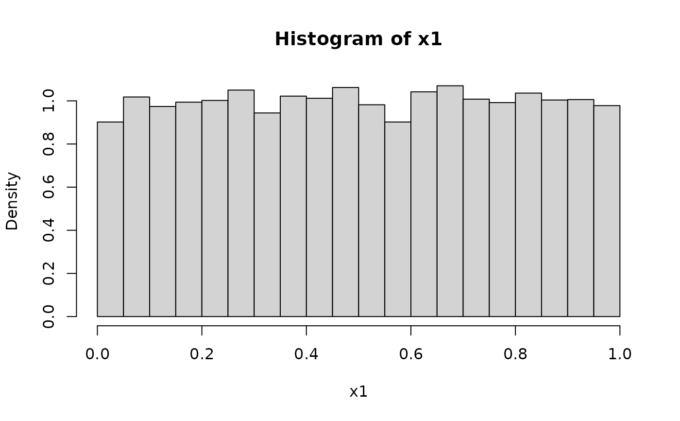
# sample from continuous uniform distribution
x1 = runif(10000)
hist(x1, xlim=c(0,1), freq=FALSE)


# discretize into 10 categories
y1 = discretize(x1, numBins=10, r=c(0,1))
y1
#> 
#>   [0,0.1] (0.1,0.2] (0.2,0.3] (0.3,0.4] (0.4,0.5] (0.5,0.6] (0.6,0.7] (0.7,0.8] 
#>       960       984      1026       983      1037       942      1056      1000 
#> (0.8,0.9]   (0.9,1] 
#>      1020       992 

# compute entropy from counts
entropy(y1) # empirical estimate near theoretical maximum
#> [1] 2.302027
log(10) # theoretical value for discrete uniform distribution with 10 bins 
#> [1] 2.302585

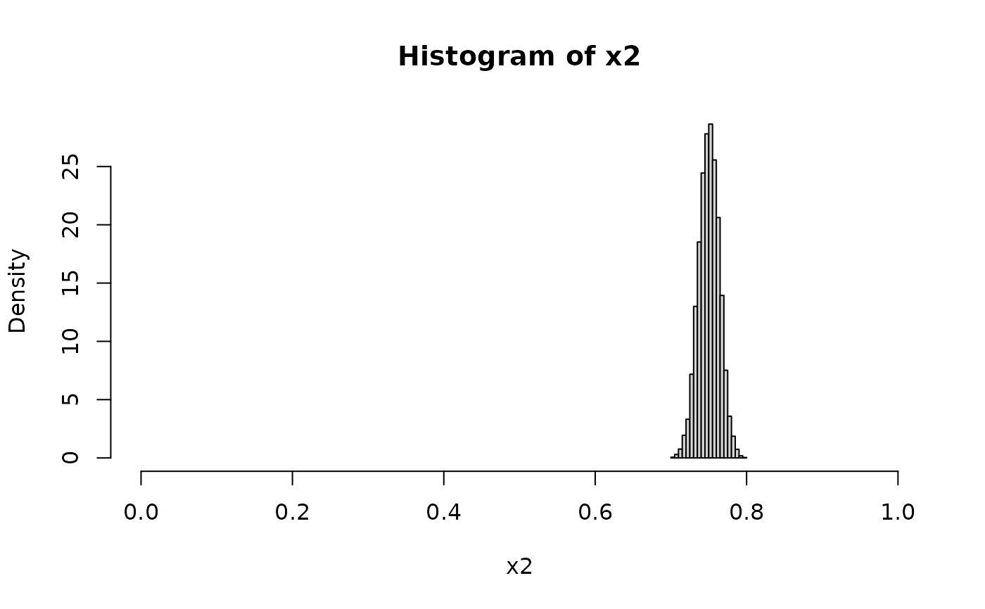
# sample from a non-uniform distribution 
x2 = rbeta(10000, 750, 250)
hist(x2, xlim=c(0,1), freq=FALSE)


# discretize into 10 categories and estimate entropy
y2 = discretize(x2, numBins=10, r=c(0,1))
y2
#> 
#>   [0,0.1] (0.1,0.2] (0.2,0.3] (0.3,0.4] (0.4,0.5] (0.5,0.6] (0.6,0.7] (0.7,0.8] 
#>         0         0         0         0         0         0         0     10000 
#> (0.8,0.9]   (0.9,1] 
#>         0         0 
entropy(y2) # almost zero
#> [1] 0

### 2D example ####

# two independent random variables
x1 = runif(10000)
x2 = runif(10000)

y2d = discretize2d(x1, x2, numBins1=10, numBins2=10)
sum(y2d)
#> [1] 10000

# joint entropy
H12 = entropy(y2d )
H12
#> [1] 4.600044
log(100) # theoretical maximum for 10x10 table
#> [1] 4.60517

# mutual information
mi.empirical(y2d) # approximately zero
#> [1] 0.004318825


# another way to compute mutual information

# compute marginal entropies
H1 = entropy(rowSums(y2d))
H2 = entropy(colSums(y2d))

H1+H2-H12 # mutual entropy
#> [1] 0.004318825