Symmetry Tests — SymmetryTests • coin

Testing the symmetry of a numeric repeated measurements variable in a complete block design.

# S3 method for class 'formula'
sign_test(formula, data, subset = NULL, ...)
# S3 method for class 'SymmetryProblem'
sign_test(object, ...)

# S3 method for class 'formula'
wilcoxsign_test(formula, data, subset = NULL, ...)
# S3 method for class 'SymmetryProblem'
wilcoxsign_test(object, zero.method = c("Pratt", "Wilcoxon"), ...)

# S3 method for class 'formula'
friedman_test(formula, data, subset = NULL, ...)
# S3 method for class 'SymmetryProblem'
friedman_test(object, ...)

# S3 method for class 'formula'
quade_test(formula, data, subset = NULL, ...)
# S3 method for class 'SymmetryProblem'
quade_test(object, ...)

Arguments

formula: a formula of the form y ~ x | block where y is a numeric variable, x is a factor with two (sign_test and wilcoxsign_test) or more levels and block is an optional factor (which is generated automatically if omitted).
data: an optional data frame containing the variables in the model formula.
subset: an optional vector specifying a subset of observations to be used. Defaults to NULL.
object: an object inheriting from class "SymmetryProblem".
zero.method: a character, the method used to handle zeros: either "Pratt" (default) or "Wilcoxon"; see ‘Details’.
...: further arguments to be passed to symmetry_test().

Details

sign_test(), wilcoxsign_test(), friedman_test() and quade_test() provide the sign test, the Wilcoxon signed-rank test, the Friedman test, the Page test and the Quade test. A general description of these methods is given by Hollander and Wolfe (1999).

The null hypothesis of symmetry is tested. The response variable and the measurement conditions are given by y and x, respectively, and block is a factor where each level corresponds to exactly one subject with repeated measurements. For sign_test and wilcoxsign_test, formulae of the form y ~ x | block and y ~ x are allowed. The latter form is interpreted as y is the first and x the second measurement on the same subject.

If x is an ordered factor, the default scores, 1:nlevels(x), can be altered using the scores argument (see symmetry_test()); this argument can also be used to coerce nominal factors to class "ordered". In this case, a linear-by-linear association test is computed and the direction of the alternative hypothesis can be specified using the alternative argument. For the Friedman test, this extension was given by Page (1963) and is known as the Page test.

For wilcoxsign_test(), the default method of handling zeros (zero.method = "Pratt"), due to Pratt (1959), first rank-transforms the absolute differences (including zeros) and then discards the ranks corresponding to the zero-differences. The proposal by Wilcoxon (1949, p. 6) first discards the zero-differences and then rank-transforms the remaining absolute differences (zero.method = "Wilcoxon").

The conditional null distribution of the test statistic is used to obtain \(p\)-values and an asymptotic approximation of the exact distribution is used by default (distribution = "asymptotic"). Alternatively, the distribution can be approximated via Monte Carlo resampling or computed exactly for univariate two-sample problems by setting distribution to "approximate" or "exact", respectively. See asymptotic(), approximate() and exact() for details.

Value

An object inheriting from class "IndependenceTest".

Note

Starting with coin version 1.0-16, the zero.method argument replaced the (now removed) ties.method argument. The current default is zero.method = "Pratt" whereas earlier versions had ties.method = "HollanderWolfe", which is equivalent to zero.method = "Wilcoxon".

References

Hollander, M. and Wolfe, D. A. (1999). Nonparametric Statistical Methods, Second Edition. New York: John Wiley & Sons.

Page, E. B. (1963). Ordered hypotheses for multiple treatments: a significance test for linear ranks. Journal of the American Statistical Association 58(301), 216–230. doi:10.1080/01621459.1963.10500843

Pratt, J. W. (1959). Remarks on zeros and ties in the Wilcoxon signed rank procedures. Journal of the American Statistical Association 54(287), 655–667. doi:10.1080/01621459.1959.10501526

Quade, D. (1979). Using weighted rankings in the analysis of complete blocks with additive block effects. Journal of the American Statistical Association 74(367), 680–683. doi:10.1080/01621459.1979.10481670

Wilcoxon, F. (1949). Some Rapid Approximate Statistical Procedures. New York: American Cyanamid Company.

Examples

## Example data from ?wilcox.test
y1 <- c(1.83,  0.50,  1.62,  2.48, 1.68, 1.88, 1.55, 3.06, 1.30)
y2 <- c(0.878, 0.647, 0.598, 2.05, 1.06, 1.29, 1.06, 3.14, 1.29)

## One-sided exact sign test
(st <- sign_test(y1 ~ y2, distribution = "exact",
                 alternative = "greater"))
#> 
#> 	Exact Sign Test
#> 
#> data:  y by x (pos, neg) 
#> 	 stratified by block
#> Z = 1.6667, p-value = 0.08984
#> alternative hypothesis: true mu is greater than 0
#> 
midpvalue(st) # mid-p-value
#> [1] 0.0546875

## One-sided exact Wilcoxon signed-rank test
(wt <- wilcoxsign_test(y1 ~ y2, distribution = "exact",
                       alternative = "greater"))
#> 
#> 	Exact Wilcoxon-Pratt Signed-Rank Test
#> 
#> data:  y by x (pos, neg) 
#> 	 stratified by block
#> Z = 2.0732, p-value = 0.01953
#> alternative hypothesis: true mu is greater than 0
#> 
statistic(wt, type = "linear")
#>       
#> pos 40
midpvalue(wt) # mid-p-value
#> [1] 0.01660156

## Comparison with R's wilcox.test() function
wilcox.test(y1, y2, paired = TRUE, alternative = "greater")
#> 
#> 	Wilcoxon signed rank exact test
#> 
#> data:  y1 and y2
#> V = 40, p-value = 0.01953
#> alternative hypothesis: true location shift is greater than 0
#> 


## Data with explicit group and block information
dta <- data.frame(y = c(y1, y2), x = gl(2, length(y1)),
                  block = factor(rep(seq_along(y1), 2)))

## For two samples, the sign test is equivalent to the Friedman test...
sign_test(y ~ x | block, data = dta, distribution = "exact")
#> 
#> 	Exact Sign Test
#> 
#> data:  y by x (pos, neg) 
#> 	 stratified by block
#> Z = 1.6667, p-value = 0.1797
#> alternative hypothesis: true mu is not equal to 0
#> 
friedman_test(y ~ x | block, data = dta, distribution = "exact")
#> 
#> 	Exact Friedman Test
#> 
#> data:  y by x (1, 2) 
#> 	 stratified by block
#> chi-squared = 2.7778, p-value = 0.1797
#> 

## ...and the signed-rank test is equivalent to the Quade test
wilcoxsign_test(y ~ x | block, data = dta, distribution = "exact")
#> 
#> 	Exact Wilcoxon-Pratt Signed-Rank Test
#> 
#> data:  y by x (pos, neg) 
#> 	 stratified by block
#> Z = 2.0732, p-value = 0.03906
#> alternative hypothesis: true mu is not equal to 0
#> 
quade_test(y ~ x | block, data = dta, distribution = "exact")
#> 
#> 	Exact Quade Test
#> 
#> data:  y by x (1, 2) 
#> 	 stratified by block
#> chi-squared = 4.2982, p-value = 0.03906
#> 


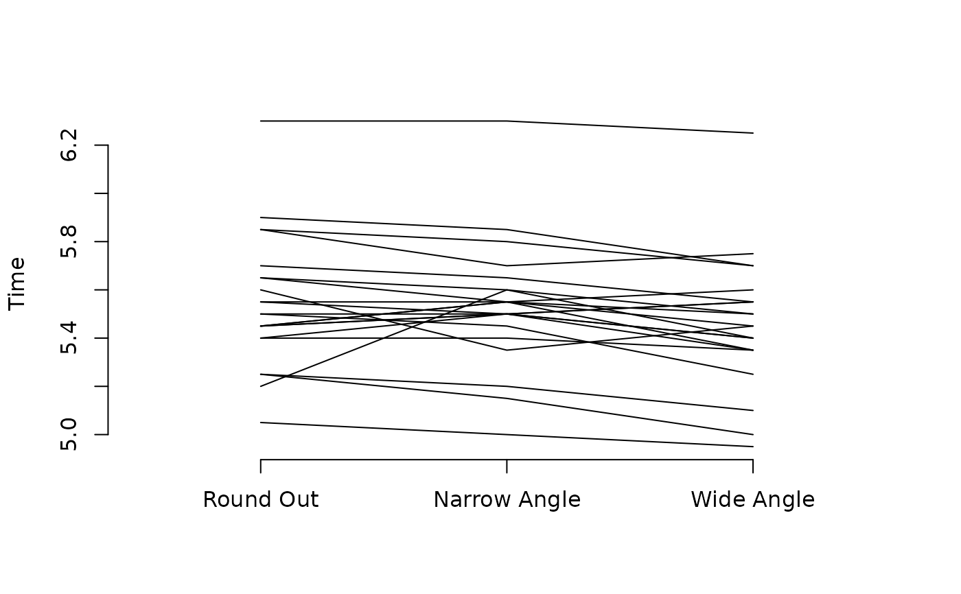
## Comparison of three methods ("round out", "narrow angle", and "wide angle")
## for rounding first base.
## Hollander and Wolfe (1999, p. 274, Tab. 7.1)
rounding <- data.frame(
    times = c(5.40, 5.50, 5.55,
              5.85, 5.70, 5.75,
              5.20, 5.60, 5.50,
              5.55, 5.50, 5.40,
              5.90, 5.85, 5.70,
              5.45, 5.55, 5.60,
              5.40, 5.40, 5.35,
              5.45, 5.50, 5.35,
              5.25, 5.15, 5.00,
              5.85, 5.80, 5.70,
              5.25, 5.20, 5.10,
              5.65, 5.55, 5.45,
              5.60, 5.35, 5.45,
              5.05, 5.00, 4.95,
              5.50, 5.50, 5.40,
              5.45, 5.55, 5.50,
              5.55, 5.55, 5.35,
              5.45, 5.50, 5.55,
              5.50, 5.45, 5.25,
              5.65, 5.60, 5.40,
              5.70, 5.65, 5.55,
              6.30, 6.30, 6.25),
    methods = factor(rep(1:3, 22),
                     labels = c("Round Out", "Narrow Angle", "Wide Angle")),
    block = gl(22, 3)
)

## Asymptotic Friedman test
friedman_test(times ~ methods | block, data = rounding)
#> 
#> 	Asymptotic Friedman Test
#> 
#> data:  times by
#> 	 methods (Round Out, Narrow Angle, Wide Angle) 
#> 	 stratified by block
#> chi-squared = 11.143, df = 2, p-value = 0.003805
#> 

## Parallel coordinates plot
with(rounding, {
    matplot(t(matrix(times, ncol = 3, byrow = TRUE)),
            type = "l", lty = 1, col = 1, ylab = "Time", xlim = c(0.5, 3.5),
            axes = FALSE)
    axis(1, at = 1:3, labels = levels(methods))
    axis(2)
})


## Where do the differences come from?
## Wilcoxon-Nemenyi-McDonald-Thompson test (Hollander and Wolfe, 1999, p. 295)
## Note: all pairwise comparisons
(st <- symmetry_test(times ~ methods | block, data = rounding,
                     ytrafo = function(data)
                         trafo(data, numeric_trafo = rank_trafo,
                               block = rounding$block),
                     xtrafo = mcp_trafo(methods = "Tukey")))
#> 
#> 	Asymptotic General Symmetry Test
#> 
#> data:  times by
#> 	 methods (Round Out, Narrow Angle, Wide Angle) 
#> 	 stratified by block
#> maxT = 3.2404, p-value = 0.00346
#> alternative hypothesis: two.sided
#> 

## Simultaneous test of all pairwise comparisons
## Wide Angle vs. Round Out differ (Hollander and Wolfe, 1999, p. 296)
pvalue(st, method = "single-step") # subset pivotality is violated
#> Warning: p-values may be incorrect due to violation
#>   of the subset pivotality condition
#>                                      
#> Narrow Angle - Round Out  0.623910827
#> Wide Angle - Round Out    0.003516106
#> Wide Angle - Narrow Angle 0.053953055


## Strength Index of Cotton
## Hollander and Wolfe (1999, p. 286, Tab. 7.5)
cotton <- data.frame(
    strength = c(7.46, 7.17, 7.76, 8.14, 7.63,
                 7.68, 7.57, 7.73, 8.15, 8.00,
                 7.21, 7.80, 7.74, 7.87, 7.93),
    potash = ordered(rep(c(144, 108, 72, 54, 36), 3),
                     levels = c(144, 108, 72, 54, 36)),
    block = gl(3, 5)
)

## One-sided asymptotic Page test
friedman_test(strength ~ potash | block, data = cotton, alternative = "greater")
#> 
#> 	Asymptotic Page Test
#> 
#> data:  strength by
#> 	 potash (144 < 108 < 72 < 54 < 36) 
#> 	 stratified by block
#> Z = 2.6558, p-value = 0.003956
#> alternative hypothesis: greater
#> 

## One-sided approximative (Monte Carlo) Page test
friedman_test(strength ~ potash | block, data = cotton, alternative = "greater",
              distribution = approximate(nresample = 10000))
#> 
#> 	Approximative Page Test
#> 
#> data:  strength by
#> 	 potash (144 < 108 < 72 < 54 < 36) 
#> 	 stratified by block
#> Z = 2.6558, p-value = 0.0023
#> alternative hypothesis: greater
#> 


## Data from Quade (1979, p. 683)
dta <- data.frame(
    y = c(52, 45, 38,
          63, 79, 50,
          45, 57, 39,
          53, 51, 43,
          47, 50, 56,
          62, 72, 49,
          49, 52, 40),
     x = factor(rep(LETTERS[1:3], 7)),
     b = factor(rep(1:7, each = 3))
)

## Approximative (Monte Carlo) Friedman test
## Quade (1979, p. 683)
friedman_test(y ~ x | b, data = dta,
              distribution = approximate(nresample = 10000)) # chi^2 = 6.000
#> 
#> 	Approximative Friedman Test
#> 
#> data:  y by x (A, B, C) 
#> 	 stratified by b
#> chi-squared = 6, p-value = 0.048
#> 

## Approximative (Monte Carlo) Quade test
## Quade (1979, p. 683)
(qt <- quade_test(y ~ x | b, data = dta,
                  distribution = approximate(nresample = 10000))) # W = 8.157
#> 
#> 	Approximative Quade Test
#> 
#> data:  y by x (A, B, C) 
#> 	 stratified by b
#> chi-squared = 8.1571, p-value = 0.0046
#> 

## Comparison with R's quade.test() function
quade.test(y ~ x | b, data = dta)
#> 
#> 	Quade test
#> 
#> data:  y and x and b
#> Quade F = 8.3765, num df = 2, denom df = 12, p-value = 0.005284
#> 

## quade.test() uses an F-statistic
b <- nlevels(qt@statistic@block)
A <- sum(qt@statistic@ytrans^2)
B <- sum(statistic(qt, type = "linear")^2) / b
(b - 1) * B / (A - B) # F = 8.3765
#> [1] 8.376528