Two- and \(K\)-Sample Location Tests
LocationTests.RdTesting the equality of the distributions of a numeric response variable in two or more independent groups against shift alternatives.
# S3 method for class 'formula'
oneway_test(formula, data, subset = NULL, weights = NULL, ...)
# S3 method for class 'IndependenceProblem'
oneway_test(object, ...)

# S3 method for class 'formula'
wilcox_test(formula, data, subset = NULL, weights = NULL, ...)
# S3 method for class 'IndependenceProblem'
wilcox_test(object, conf.int = FALSE, conf.level = 0.95, ...)

# S3 method for class 'formula'
kruskal_test(formula, data, subset = NULL, weights = NULL, ...)
# S3 method for class 'IndependenceProblem'
kruskal_test(object, ...)

# S3 method for class 'formula'
normal_test(formula, data, subset = NULL, weights = NULL, ...)
# S3 method for class 'IndependenceProblem'
normal_test(object, ties.method = c("mid-ranks", "average-scores"),
            conf.int = FALSE, conf.level = 0.95, ...)

# S3 method for class 'formula'
median_test(formula, data, subset = NULL, weights = NULL, ...)
# S3 method for class 'IndependenceProblem'
median_test(object, mid.score = c("0", "0.5", "1"),
            conf.int = FALSE, conf.level = 0.95, ...)

# S3 method for class 'formula'
savage_test(formula, data, subset = NULL, weights = NULL, ...)
# S3 method for class 'IndependenceProblem'
savage_test(object, ties.method = c("mid-ranks", "average-scores"),
            conf.int = FALSE, conf.level = 0.95, ...)
Arguments
- formula
a formula of the form
y ~ x | blockwhereyis a numeric variable,xis a factor andblockis an optional factor for stratification.- data
an optional data frame containing the variables in the model formula.
- subset
an optional vector specifying a subset of observations to be used. Defaults to
NULL.- weights
an optional formula of the form
~ wdefining integer valued case weights for each observation. Defaults toNULL, implying equal weight for all observations.- object
an object inheriting from class
"IndependenceProblem".- conf.int
a logical indicating whether a confidence interval for the difference in location should be computed. Defaults to
FALSE.- conf.level
a numeric, confidence level of the interval. Defaults to
0.95.- ties.method
a character, the method used to handle ties: the score generating function either uses mid-ranks (
"mid-ranks", default) or averages the scores of randomly broken ties ("average-scores").- mid.score
a character, the score assigned to observations exactly equal to the median: either 0 (
"0", default), 0.5 ("0.5") or 1 ("1"); see ‘Details’.- ...
further arguments to be passed to
independence_test().
Details
oneway_test(), wilcox_test(), kruskal_test(),
normal_test(), median_test() and savage_test() provide
the Fisher-Pitman permutation test, the Wilcoxon-Mann-Whitney test, the
Kruskal-Wallis test, the van der Waerden test, the Brown-Mood median test and
the Savage test. A general description of these methods is given by Hollander
and Wolfe (1999). For the adjustment of scores for tied values see
Hájek, Šidák and Sen (1999, pp. 133–135).
The null hypothesis of equality, or conditional equality given block,
of the distribution of y in the groups defined by x is tested
against shift alternatives. In the two-sample case, the two-sided null
hypothesis is \(H_0\!: \mu = 0\), where \(\mu = Y_1 - Y_2\)
and \(Y_s\) is the median of the responses in the \(s\)th sample. In case
alternative = "less", the null hypothesis is \(H_0\!: \mu \ge
0\). When alternative = "greater", the null hypothesis
is \(H_0\!: \mu \le 0\). Confidence intervals for the
difference in location are available (except for oneway_test()) and
computed according to Bauer (1972).
If x is an ordered factor, the default scores, 1:nlevels(x), can
be altered using the scores argument (see
independence_test()); this argument can also be used to coerce
nominal factors to class "ordered". In this case, a linear-by-linear
association test is computed and the direction of the alternative hypothesis
can be specified using the alternative argument.
The Brown-Mood median test offers a choice of mid-score, i.e., the score
assigned to observations exactly equal to the median. In the two-sample case,
mid-score = "0" implies that the linear test statistic is simply the
number of subjects in the second sample with observations greater than the
median of the pooled sample. Similarly, the linear test statistic for the
last alternative, mid-score = "1", is the number of subjects in the
second sample with observations greater than or equal to the median of the
pooled sample. If mid-score = "0.5" is selected, the linear test
statistic is the mean of the test statistics corresponding to the first and
last alternatives and has a symmetric distribution, or at least approximately
so, under the null hypothesis (see Hájek, Šidák
and Sen, 1999, pp. 97–98).
The conditional null distribution of the test statistic is used to obtain
\(p\)-values and an asymptotic approximation of the exact distribution is
used by default (distribution = "asymptotic"). Alternatively, the
distribution can be approximated via Monte Carlo resampling or computed
exactly for univariate two-sample problems by setting distribution to
"approximate" or "exact", respectively. See
asymptotic(), approximate() and
exact() for details.
Value
An object inheriting from class "IndependenceTest".
Confidence intervals can be extracted by confint().
Note
Starting with coin version 1.1-0, oneway_test() no longer allows
the test statistic to be specified; a quadratic form is now used in the
\(K\)-sample case. Please use independence_test() if more
control is desired.
References
Bauer, D. F. (1972). Constructing confidence sets using rank statistics. Journal of the American Statistical Association 67(339), 687–690. doi:10.1080/01621459.1972.10481279
Hájek, J., Šidák, Z. and Sen, P. K. (1999). Theory of Rank Tests, Second Edition. San Diego: Academic Press.
Hollander, M. and Wolfe, D. A. (1999). Nonparametric Statistical Methods, Second Edition. New York: John Wiley & Sons.
Examples
## Tritiated Water Diffusion Across Human Chorioamnion
## Hollander and Wolfe (1999, p. 110, Tab. 4.1)
diffusion <- data.frame(
pd = c(0.80, 0.83, 1.89, 1.04, 1.45, 1.38, 1.91, 1.64, 0.73, 1.46,
1.15, 0.88, 0.90, 0.74, 1.21),
age = factor(rep(c("At term", "12-26 Weeks"), c(10, 5)))
)
## Exact Wilcoxon-Mann-Whitney test
## Hollander and Wolfe (1999, p. 111)
## (At term - 12-26 Weeks)
(wt <- wilcox_test(pd ~ age, data = diffusion,
distribution = "exact", conf.int = TRUE))
#>
#> Exact Wilcoxon-Mann-Whitney Test
#>
#> data: pd by age (12-26 Weeks, At term)
#> Z = -1.2247, p-value = 0.2544
#> alternative hypothesis: true mu is not equal to 0
#> 95 percent confidence interval:
#> -0.76 0.15
#> sample estimates:
#> difference in location
#> -0.305
#>
## Extract observed Wilcoxon statistic
## Note: this is the sum of the ranks for age = "12-26 Weeks"
statistic(wt, type = "linear")
#>
#> 12-26 Weeks 30
## Expectation, variance, two-sided pvalue and confidence interval
expectation(wt)
#>
#> 12-26 Weeks 40
covariance(wt)
#> 12-26 Weeks
#> 12-26 Weeks 66.66667
pvalue(wt)
#> [1] 0.2544123
confint(wt)
#> 95 percent confidence interval:
#> -0.76 0.15
#> sample estimates:
#> difference in location
#> -0.305
#>
## For two samples, the Kruskal-Wallis test is equivalent to the W-M-W test
kruskal_test(pd ~ age, data = diffusion,
distribution = "exact")
#>
#> Exact Kruskal-Wallis Test
#>
#> data: pd by age (12-26 Weeks, At term)
#> chi-squared = 1.5, p-value = 0.2544
#>
## Asymptotic Fisher-Pitman test
oneway_test(pd ~ age, data = diffusion)
#>
#> Asymptotic Two-Sample Fisher-Pitman Permutation Test
#>
#> data: pd by age (12-26 Weeks, At term)
#> Z = -1.5225, p-value = 0.1279
#> alternative hypothesis: true mu is not equal to 0
#>
## Approximative (Monte Carlo) Fisher-Pitman test
pvalue(oneway_test(pd ~ age, data = diffusion,
distribution = approximate(nresample = 10000)))
#> [1] 0.1372
#> 99 percent confidence interval:
#> 0.1284623 0.1462855
#>
## Exact Fisher-Pitman test
pvalue(ot <- oneway_test(pd ~ age, data = diffusion,
distribution = "exact"))
#> [1] 0.1318681
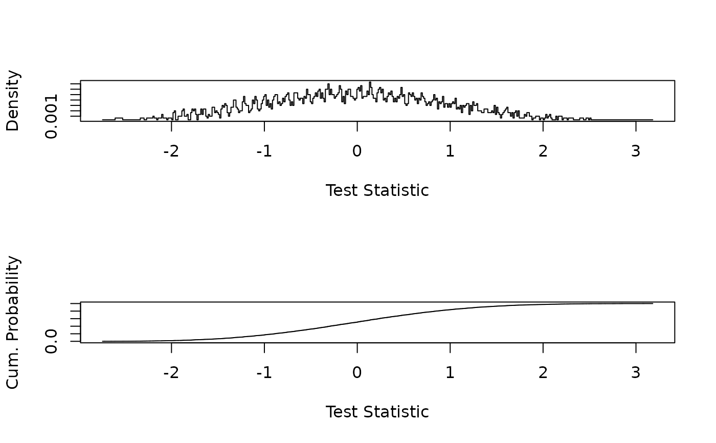
## Plot density and distribution of the standardized test statistic
op <- par(no.readonly = TRUE) # save current settings
layout(matrix(1:2, nrow = 2))
s <- support(ot)
d <- dperm(ot, s)
p <- pperm(ot, s)
plot(s, d, type = "S", xlab = "Test Statistic", ylab = "Density")
plot(s, p, type = "S", xlab = "Test Statistic", ylab = "Cum. Probability")
 par(op) # reset
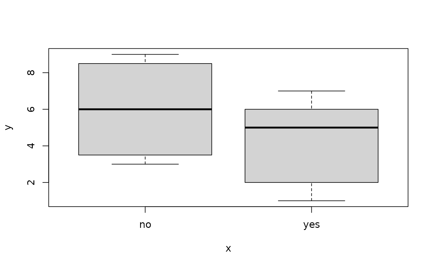
## Example data
ex <- data.frame(
y = c(3, 4, 8, 9, 1, 2, 5, 6, 7),
x = factor(rep(c("no", "yes"), c(4, 5)))
)
## Boxplots
boxplot(y ~ x, data = ex)
par(op) # reset
## Example data
ex <- data.frame(
y = c(3, 4, 8, 9, 1, 2, 5, 6, 7),
x = factor(rep(c("no", "yes"), c(4, 5)))
)
## Boxplots
boxplot(y ~ x, data = ex)
 ## Exact Brown-Mood median test with different mid-scores
(mt1 <- median_test(y ~ x, data = ex, distribution = "exact"))
#>
#> Exact Two-Sample Brown-Mood Median Test
#>
#> data: y by x (no, yes)
#> Z = 0.28284, p-value = 1
#> alternative hypothesis: true mu is not equal to 0
#>
(mt2 <- median_test(y ~ x, data = ex, distribution = "exact",
mid.score = "0.5"))
#>
#> Exact Two-Sample Brown-Mood Median Test
#>
#> data: y by x (no, yes)
#> Z = 0, p-value = 1
#> alternative hypothesis: true mu is not equal to 0
#>
(mt3 <- median_test(y ~ x, data = ex, distribution = "exact",
mid.score = "1")) # sign change!
#>
#> Exact Two-Sample Brown-Mood Median Test
#>
#> data: y by x (no, yes)
#> Z = -0.28284, p-value = 1
#> alternative hypothesis: true mu is not equal to 0
#>
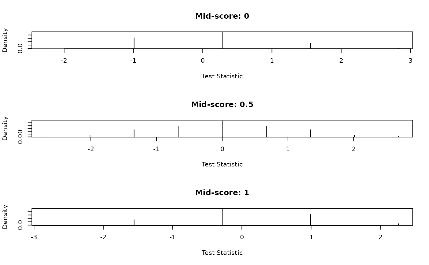
## Plot density and distribution of the standardized test statistics
op <- par(no.readonly = TRUE) # save current settings
layout(matrix(1:3, nrow = 3))
s1 <- support(mt1); d1 <- dperm(mt1, s1)
plot(s1, d1, type = "h", main = "Mid-score: 0",
xlab = "Test Statistic", ylab = "Density")
s2 <- support(mt2); d2 <- dperm(mt2, s2)
plot(s2, d2, type = "h", main = "Mid-score: 0.5",
xlab = "Test Statistic", ylab = "Density")
s3 <- support(mt3); d3 <- dperm(mt3, s3)
plot(s3, d3, type = "h", main = "Mid-score: 1",
xlab = "Test Statistic", ylab = "Density")
## Exact Brown-Mood median test with different mid-scores
(mt1 <- median_test(y ~ x, data = ex, distribution = "exact"))
#>
#> Exact Two-Sample Brown-Mood Median Test
#>
#> data: y by x (no, yes)
#> Z = 0.28284, p-value = 1
#> alternative hypothesis: true mu is not equal to 0
#>
(mt2 <- median_test(y ~ x, data = ex, distribution = "exact",
mid.score = "0.5"))
#>
#> Exact Two-Sample Brown-Mood Median Test
#>
#> data: y by x (no, yes)
#> Z = 0, p-value = 1
#> alternative hypothesis: true mu is not equal to 0
#>
(mt3 <- median_test(y ~ x, data = ex, distribution = "exact",
mid.score = "1")) # sign change!
#>
#> Exact Two-Sample Brown-Mood Median Test
#>
#> data: y by x (no, yes)
#> Z = -0.28284, p-value = 1
#> alternative hypothesis: true mu is not equal to 0
#>
## Plot density and distribution of the standardized test statistics
op <- par(no.readonly = TRUE) # save current settings
layout(matrix(1:3, nrow = 3))
s1 <- support(mt1); d1 <- dperm(mt1, s1)
plot(s1, d1, type = "h", main = "Mid-score: 0",
xlab = "Test Statistic", ylab = "Density")
s2 <- support(mt2); d2 <- dperm(mt2, s2)
plot(s2, d2, type = "h", main = "Mid-score: 0.5",
xlab = "Test Statistic", ylab = "Density")
s3 <- support(mt3); d3 <- dperm(mt3, s3)
plot(s3, d3, type = "h", main = "Mid-score: 1",
xlab = "Test Statistic", ylab = "Density")
 par(op) # reset
## Length of YOY Gizzard Shad
## Hollander and Wolfe (1999, p. 200, Tab. 6.3)
yoy <- data.frame(
length = c(46, 28, 46, 37, 32, 41, 42, 45, 38, 44,
42, 60, 32, 42, 45, 58, 27, 51, 42, 52,
38, 33, 26, 25, 28, 28, 26, 27, 27, 27,
31, 30, 27, 29, 30, 25, 25, 24, 27, 30),
site = gl(4, 10, labels = as.roman(1:4))
)
## Approximative (Monte Carlo) Kruskal-Wallis test
kruskal_test(length ~ site, data = yoy,
distribution = approximate(nresample = 10000))
#>
#> Approximative Kruskal-Wallis Test
#>
#> data: length by site (I, II, III, IV)
#> chi-squared = 22.852, p-value < 1e-04
#>
## Approximative (Monte Carlo) Nemenyi-Damico-Wolfe-Dunn test (joint ranking)
## Hollander and Wolfe (1999, p. 244)
## (where Steel-Dwass results are given)
it <- independence_test(length ~ site, data = yoy,
distribution = approximate(nresample = 50000),
ytrafo = function(data)
trafo(data, numeric_trafo = rank_trafo),
xtrafo = mcp_trafo(site = "Tukey"))
## Global p-value
pvalue(it)
#> [1] 0.00044
#> 99 percent confidence interval:
#> 0.0002358587 0.0007442521
#>
## Sites (I = II) != (III = IV) at alpha = 0.01 (p. 244)
pvalue(it, method = "single-step") # subset pivotality is violated
#> Warning: p-values may be incorrect due to violation
#> of the subset pivotality condition
#>
#> II - I 0.94804
#> III - I 0.00854
#> IV - I 0.00674
#> III - II 0.00064
#> IV - II 0.00044
#> IV - III 0.99994
par(op) # reset
## Length of YOY Gizzard Shad
## Hollander and Wolfe (1999, p. 200, Tab. 6.3)
yoy <- data.frame(
length = c(46, 28, 46, 37, 32, 41, 42, 45, 38, 44,
42, 60, 32, 42, 45, 58, 27, 51, 42, 52,
38, 33, 26, 25, 28, 28, 26, 27, 27, 27,
31, 30, 27, 29, 30, 25, 25, 24, 27, 30),
site = gl(4, 10, labels = as.roman(1:4))
)
## Approximative (Monte Carlo) Kruskal-Wallis test
kruskal_test(length ~ site, data = yoy,
distribution = approximate(nresample = 10000))
#>
#> Approximative Kruskal-Wallis Test
#>
#> data: length by site (I, II, III, IV)
#> chi-squared = 22.852, p-value < 1e-04
#>
## Approximative (Monte Carlo) Nemenyi-Damico-Wolfe-Dunn test (joint ranking)
## Hollander and Wolfe (1999, p. 244)
## (where Steel-Dwass results are given)
it <- independence_test(length ~ site, data = yoy,
distribution = approximate(nresample = 50000),
ytrafo = function(data)
trafo(data, numeric_trafo = rank_trafo),
xtrafo = mcp_trafo(site = "Tukey"))
## Global p-value
pvalue(it)
#> [1] 0.00044
#> 99 percent confidence interval:
#> 0.0002358587 0.0007442521
#>
## Sites (I = II) != (III = IV) at alpha = 0.01 (p. 244)
pvalue(it, method = "single-step") # subset pivotality is violated
#> Warning: p-values may be incorrect due to violation
#> of the subset pivotality condition
#>
#> II - I 0.94804
#> III - I 0.00854
#> IV - I 0.00674
#> III - II 0.00064
#> IV - II 0.00044
#> IV - III 0.99994