Compute or Extract Silhouette Information from Clustering
silhouette.RdCompute silhouette information according to a given clustering in \(k\) clusters.
silhouette(x, ...)
# Default S3 method
silhouette  (x, dist, dmatrix, ...)
# S3 method for class 'partition'
silhouette(x, ...)
# S3 method for class 'clara'
silhouette(x, full = FALSE, subset = NULL, ...)

sortSilhouette(object, ...)
# S3 method for class 'silhouette'
summary(object, FUN = mean, ...)
# S3 method for class 'silhouette'
plot(x, nmax.lab = 40, max.strlen = 5,
     main = NULL, sub = NULL, xlab = expression("Silhouette width "* s[i]),
     col = "gray",  do.col.sort = length(col) > 1, border = 0,
     cex.names = par("cex.axis"), do.n.k = TRUE, do.clus.stat = TRUE, ...)
Arguments
- x
an object of appropriate class; for the
defaultmethod an integer vector with \(k\) different integer cluster codes or a list with such anx$clusteringcomponent. Note that silhouette statistics are only defined if \(2 \le k \le n-1\).- dist
a dissimilarity object inheriting from class
distor coercible to one. If not specified,dmatrixmust be.- dmatrix
a symmetric dissimilarity matrix (\(n \times n\)), specified instead of
dist, which can be more efficient.- full
logical or number in \([0,1]\) specifying if a full silhouette should be computed for
claraobject. When a number, say \(f\), for a randomsample.int(n, size = f*n)of the data the silhouette values are computed. This requires \(O((f*n)^2)\) memory, since the full dissimilarity of the (sub)sample (seedaisy) is needed internally.- subset
a subset from
1:n, specified instead offullto specify the indices of the observations to be used for the silhouette computations.- object
an object of class
silhouette.- ...
further arguments passed to and from methods.
- FUN
function used to summarize silhouette widths.
- nmax.lab
integer indicating the number of labels which is considered too large for single-name labeling the silhouette plot.
- max.strlen
positive integer giving the length to which strings are truncated in silhouette plot labeling.
- main, sub, xlab
arguments to
title; have a sensible non-NULL default here.- col, border, cex.names
arguments passed
barplot(); note that the default used to becol = heat.colors(n), border = par("fg")instead.colcan also be a color vector of length \(k\) for clusterwise coloring, see alsodo.col.sort:- do.col.sort
logical indicating if the colors
colshould be sorted “along” the silhouette; this is useful for casewise or clusterwise coloring.- do.n.k
logical indicating if \(n\) and \(k\) “title text” should be written.
- do.clus.stat
logical indicating if cluster size and averages should be written right to the silhouettes.
Details
For each observation i, the silhouette width \(s(i)\) is
defined as follows:
Put a(i) = average dissimilarity between i and all other points of the
cluster to which i belongs (if i is the only observation in
its cluster, \(s(i) := 0\) without further calculations).
For all other clusters C, put \(d(i,C)\) = average
dissimilarity of i to all observations of C. The smallest of these
\(d(i,C)\) is \(b(i) := \min_C d(i,C)\),
and can be seen as the dissimilarity between i and its “neighbor”
cluster, i.e., the nearest one to which it does not belong.
Finally, $$s(i) := \frac{b(i) - a(i) }{max(a(i), b(i))}.$$
silhouette.default() is now based on C code donated by Romain
Francois (the R version being still available as cluster:::silhouetteR).
Observations with a large \(s(i)\) (almost 1) are very well clustered, a small \(s(i)\) (around 0) means that the observation lies between two clusters, and observations with a negative \(s(i)\) are probably placed in the wrong cluster.
Note
While silhouette() is intrinsic to the
partition clusterings, and hence has a (trivial) method
for these, it is straightforward to get silhouettes from hierarchical
clusterings from silhouette.default() with
cutree() and distance as input.
By default, for clara() partitions, the silhouette is
just for the best random subset used. Use full = TRUE
to compute (and later possibly plot) the full silhouette.
Value
silhouette() returns an object, sil, of class
silhouette which is an \(n \times 3\) matrix with
attributes. For each observation i, sil[i,] contains the
cluster to which i belongs as well as the neighbor cluster of i (the
cluster, not containing i, for which the average dissimilarity between its
observations and i is minimal), and the silhouette width \(s(i)\) of
the observation. The colnames correspondingly are
c("cluster", "neighbor", "sil_width").
summary(sil) returns an object of class
summary.silhouette, a list with components
si.summary:numerical
summaryof the individual silhouette widths \(s(i)\).clus.avg.widths:numeric (rank 1) array of clusterwise means of silhouette widths where
mean = FUNis used.avg.width:the total mean
FUN(s)wheresare the individual silhouette widths.clus.sizes:tableof the \(k\) cluster sizes.call:if available, the
callcreatingsil.Ordered:logical identical to
attr(sil, "Ordered"), see below.
sortSilhouette(sil) orders the rows of sil as in the
silhouette plot, by cluster (increasingly) and decreasing silhouette
width \(s(i)\).
attr(sil, "Ordered") is a logical indicating if sil is
ordered as by sortSilhouette(). In that case,
rownames(sil) will contain case labels or numbers, and attr(sil, "iOrd") the ordering index vector.
References
Rousseeuw, P.J. (1987) Silhouettes: A graphical aid to the interpretation and validation of cluster analysis. J. Comput. Appl. Math., 20, 53–65.
chapter 2 of Kaufman and Rousseeuw (1990), see
the references in plot.agnes.
See also
Examples
data(ruspini)
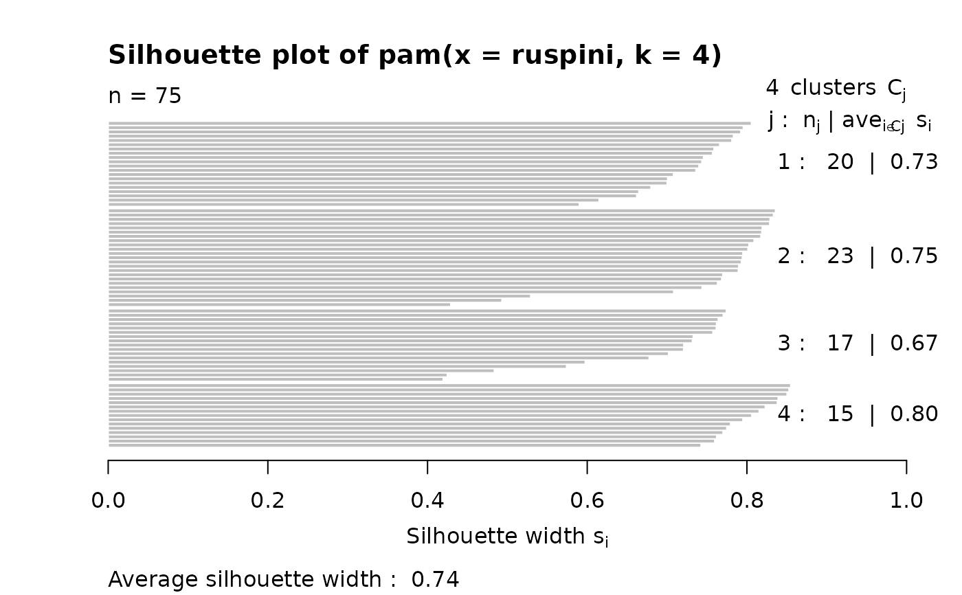
pr4 <- pam(ruspini, 4)
str(si <- silhouette(pr4))
#> 'silhouette' num [1:75, 1:3] 1 1 1 1 1 1 1 1 1 1 ...
#> - attr(*, "dimnames")=List of 2
#> ..$ : chr [1:75] "10" "6" "9" "11" ...
#> ..$ : chr [1:3] "cluster" "neighbor" "sil_width"
#> - attr(*, "Ordered")= logi TRUE
#> - attr(*, "call")= language pam(x = ruspini, k = 4)
(ssi <- summary(si))
#> Silhouette of 75 units in 4 clusters from pam(x = ruspini, k = 4) :
#> Cluster sizes and average silhouette widths:
#> 20 23 17 15
#> 0.7262347 0.7548344 0.6691154 0.8042285
#> Individual silhouette widths:
#> Min. 1st Qu. Median Mean 3rd Qu. Max.
#> 0.4196 0.7145 0.7642 0.7377 0.7984 0.8549
plot(si) # silhouette plot
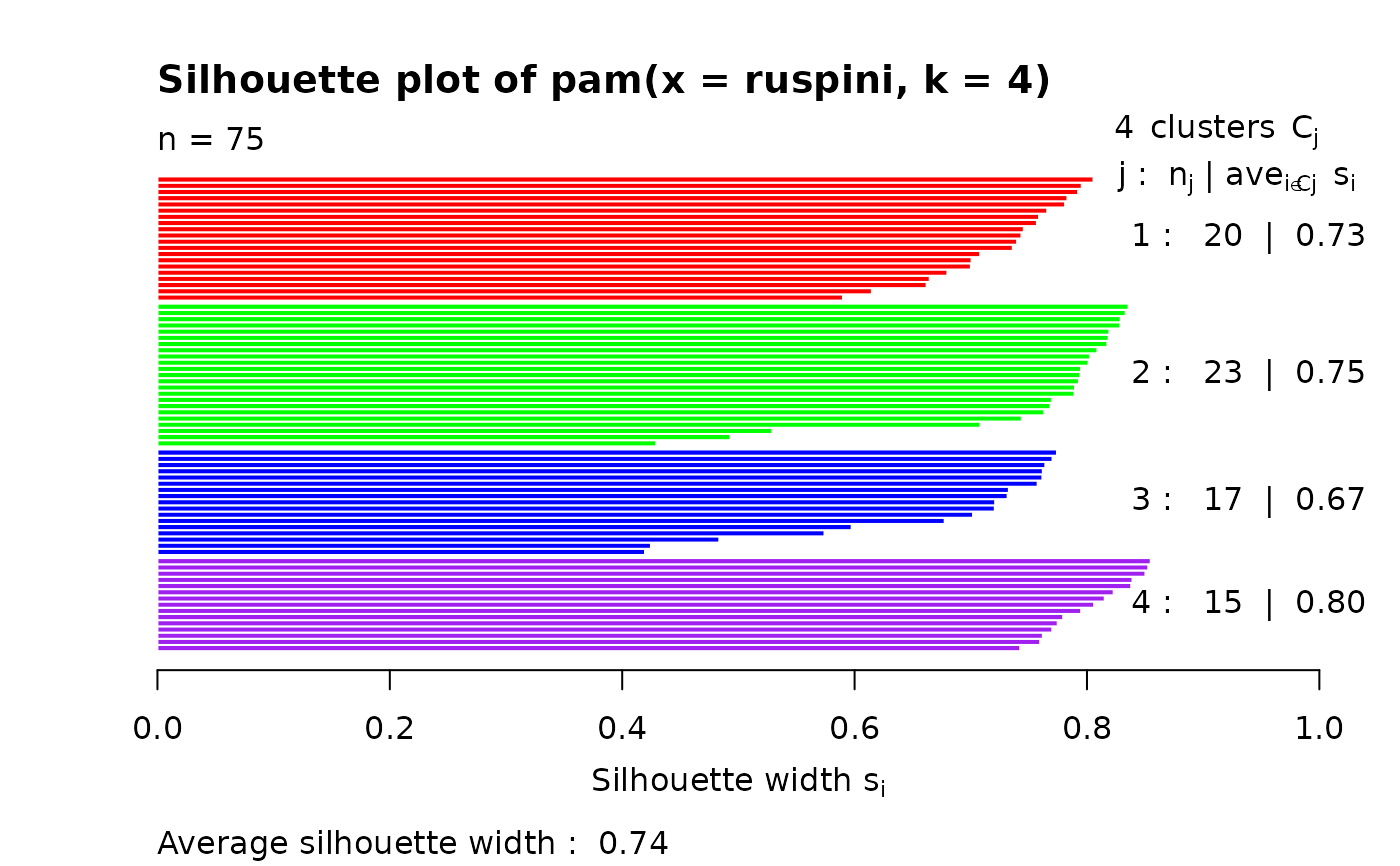
 plot(si, col = c("red", "green", "blue", "purple"))# with cluster-wise coloring
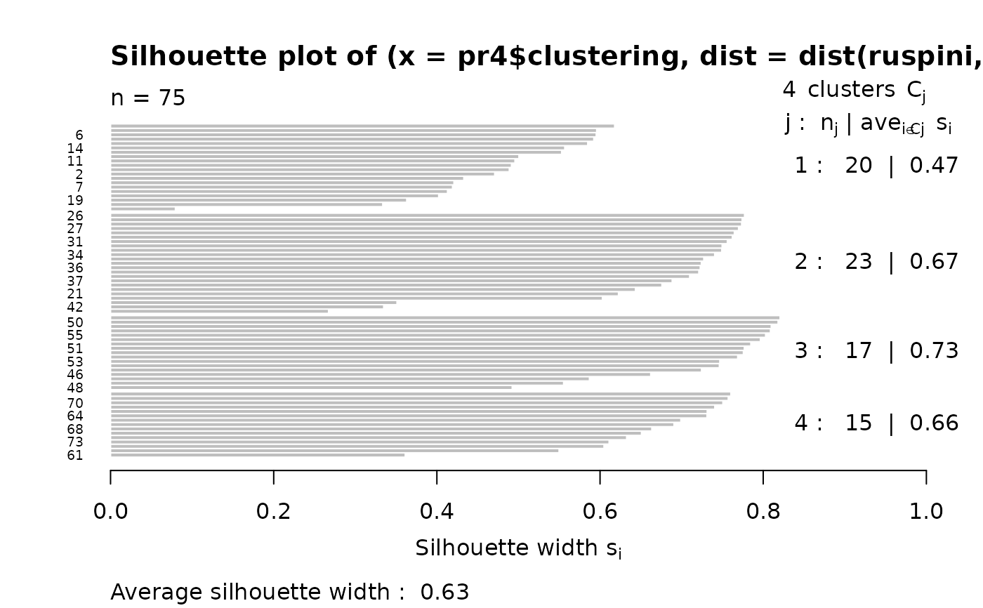
 si2 <- silhouette(pr4$clustering, dist(ruspini, "canberra"))
summary(si2) # has small values: "canberra"'s fault
#> Silhouette of 75 units in 4 clusters from silhouette.default(x = pr4$clustering, dist = dist(ruspini, "canberra")) :
#> Cluster sizes and average silhouette widths:
#> 20 23 17 15
#> 0.4704136 0.6699338 0.7339873 0.6623204
#> Individual silhouette widths:
#> Min. 1st Qu. Median Mean 3rd Qu. Max.
#> 0.07951 0.55135 0.67585 0.62972 0.75332 0.82071
plot(si2, nmax= 80, cex.names=0.6)
si2 <- silhouette(pr4$clustering, dist(ruspini, "canberra"))
summary(si2) # has small values: "canberra"'s fault
#> Silhouette of 75 units in 4 clusters from silhouette.default(x = pr4$clustering, dist = dist(ruspini, "canberra")) :
#> Cluster sizes and average silhouette widths:
#> 20 23 17 15
#> 0.4704136 0.6699338 0.7339873 0.6623204
#> Individual silhouette widths:
#> Min. 1st Qu. Median Mean 3rd Qu. Max.
#> 0.07951 0.55135 0.67585 0.62972 0.75332 0.82071
plot(si2, nmax= 80, cex.names=0.6)
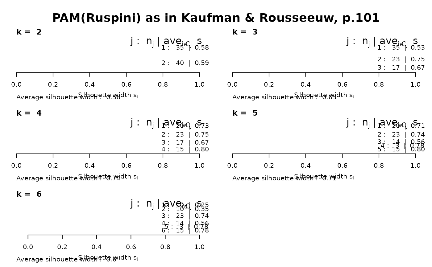
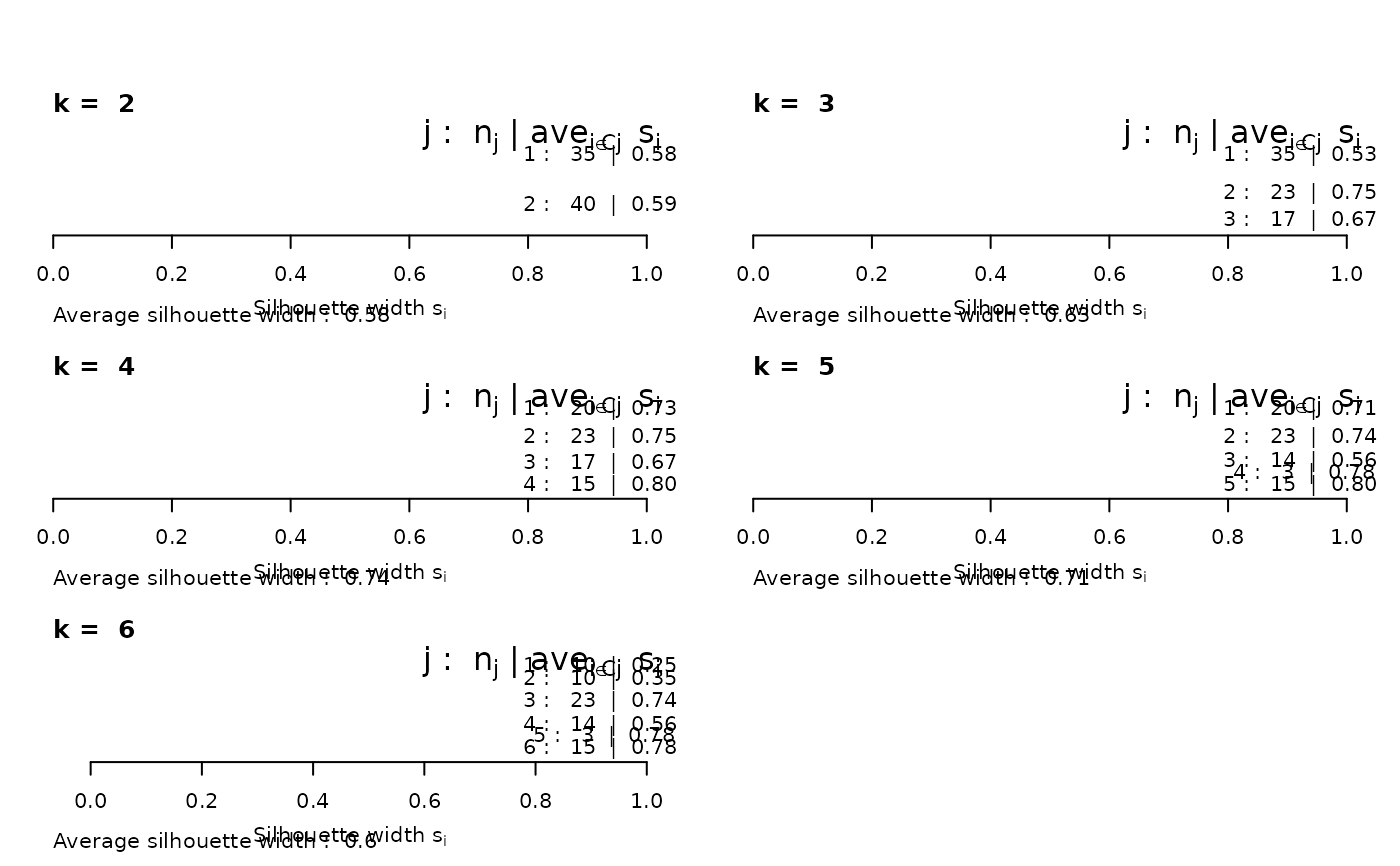
 op <- par(mfrow= c(3,2), oma= c(0,0, 3, 0),
mgp= c(1.6,.8,0), mar= .1+c(4,2,2,2))
for(k in 2:6)
plot(silhouette(pam(ruspini, k=k)), main = paste("k = ",k), do.n.k=FALSE)
mtext("PAM(Ruspini) as in Kaufman & Rousseeuw, p.101",
outer = TRUE, font = par("font.main"), cex = par("cex.main")); frame()
op <- par(mfrow= c(3,2), oma= c(0,0, 3, 0),
mgp= c(1.6,.8,0), mar= .1+c(4,2,2,2))
for(k in 2:6)
plot(silhouette(pam(ruspini, k=k)), main = paste("k = ",k), do.n.k=FALSE)
mtext("PAM(Ruspini) as in Kaufman & Rousseeuw, p.101",
outer = TRUE, font = par("font.main"), cex = par("cex.main")); frame()
 ## the same with cluster-wise colours:
c6 <- c("tomato", "forest green", "dark blue", "purple2", "goldenrod4", "gray20")
for(k in 2:6)
plot(silhouette(pam(ruspini, k=k)), main = paste("k = ",k), do.n.k=FALSE,
col = c6[1:k])
par(op)
## the same with cluster-wise colours:
c6 <- c("tomato", "forest green", "dark blue", "purple2", "goldenrod4", "gray20")
for(k in 2:6)
plot(silhouette(pam(ruspini, k=k)), main = paste("k = ",k), do.n.k=FALSE,
col = c6[1:k])
par(op)
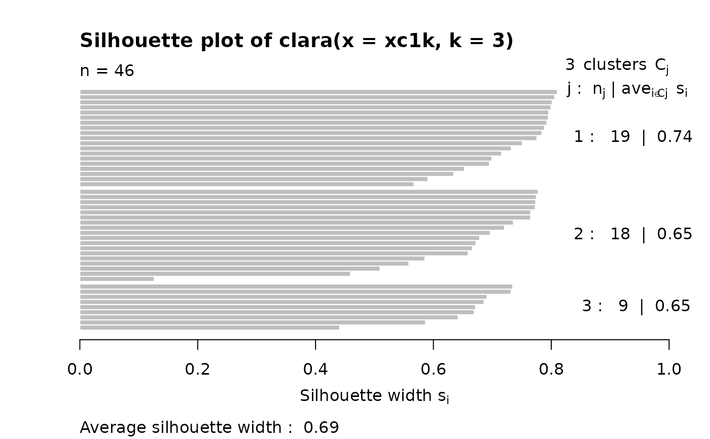
 ## clara(): standard silhouette is just for the best random subset
data(xclara)
set.seed(7)
str(xc1k <- xclara[ sample(nrow(xclara), size = 1000) ,]) # rownames == indices
#> 'data.frame': 1000 obs. of 2 variables:
#> $ V1: num 44.6 11.2 71.6 17.6 77.5 ...
#> $ V2: num 78.78 27.96 -26.88 69.15 -7.26 ...
cl3 <- clara(xc1k, 3)
plot(silhouette(cl3))# only of the "best" subset of 46
## clara(): standard silhouette is just for the best random subset
data(xclara)
set.seed(7)
str(xc1k <- xclara[ sample(nrow(xclara), size = 1000) ,]) # rownames == indices
#> 'data.frame': 1000 obs. of 2 variables:
#> $ V1: num 44.6 11.2 71.6 17.6 77.5 ...
#> $ V2: num 78.78 27.96 -26.88 69.15 -7.26 ...
cl3 <- clara(xc1k, 3)
plot(silhouette(cl3))# only of the "best" subset of 46
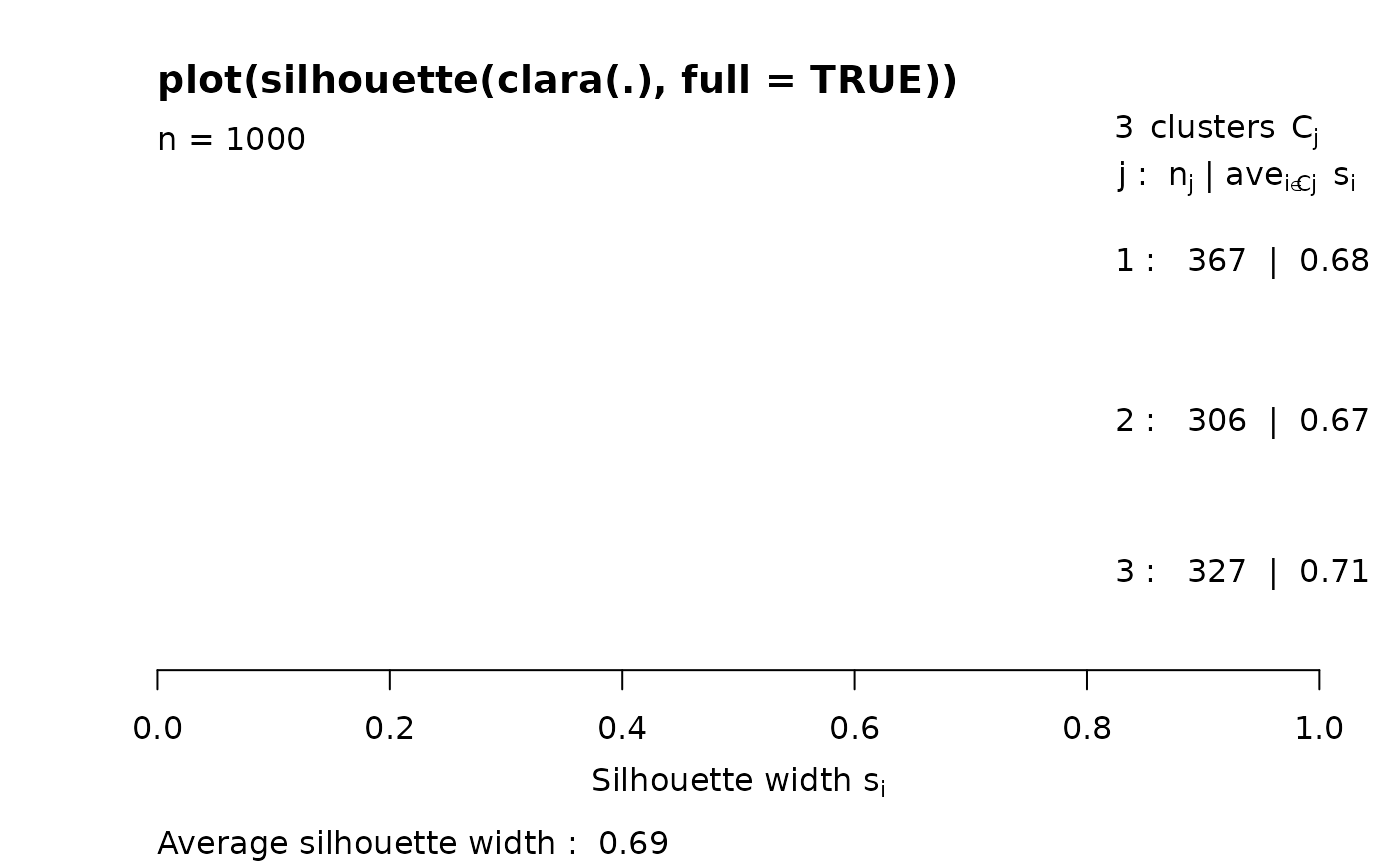
 ## The full silhouette: internally needs large (36 MB) dist object:
sf <- silhouette(cl3, full = TRUE) ## this is the same as
s.full <- silhouette(cl3$clustering, daisy(xc1k))
stopifnot(all.equal(sf, s.full, check.attributes = FALSE, tolerance = 0))
## color dependent on original "3 groups of each 1000": % __FIXME ??__
plot(sf, col = 2+ as.integer(names(cl3$clustering) ) %/% 1000,
main ="plot(silhouette(clara(.), full = TRUE))")
## The full silhouette: internally needs large (36 MB) dist object:
sf <- silhouette(cl3, full = TRUE) ## this is the same as
s.full <- silhouette(cl3$clustering, daisy(xc1k))
stopifnot(all.equal(sf, s.full, check.attributes = FALSE, tolerance = 0))
## color dependent on original "3 groups of each 1000": % __FIXME ??__
plot(sf, col = 2+ as.integer(names(cl3$clustering) ) %/% 1000,
main ="plot(silhouette(clara(.), full = TRUE))")
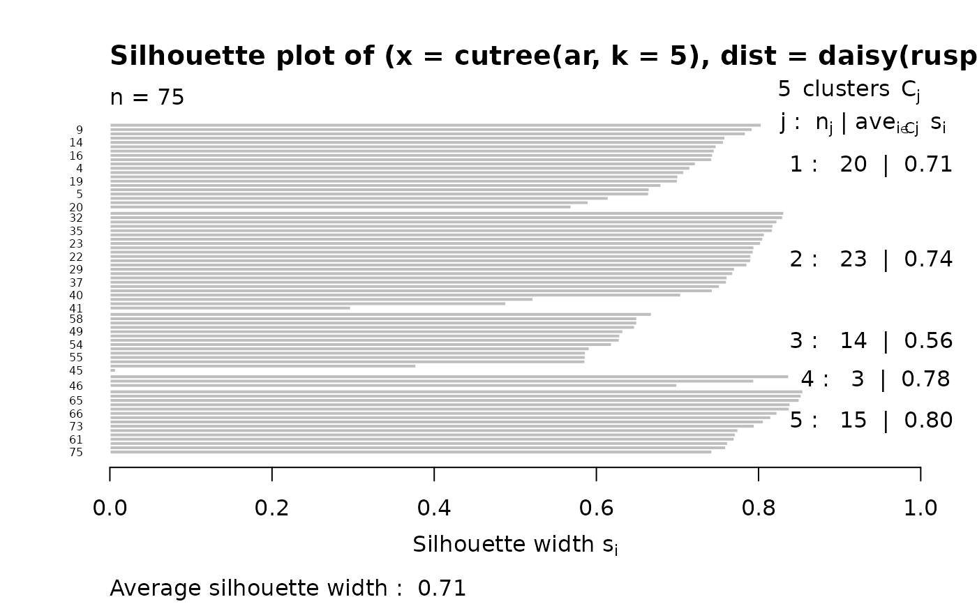
 ## Silhouette for a hierarchical clustering:
ar <- agnes(ruspini)
si3 <- silhouette(cutree(ar, k = 5), # k = 4 gave the same as pam() above
daisy(ruspini))
stopifnot(is.data.frame(di3 <- as.data.frame(si3)))
plot(si3, nmax = 80, cex.names = 0.5)
## Silhouette for a hierarchical clustering:
ar <- agnes(ruspini)
si3 <- silhouette(cutree(ar, k = 5), # k = 4 gave the same as pam() above
daisy(ruspini))
stopifnot(is.data.frame(di3 <- as.data.frame(si3)))
plot(si3, nmax = 80, cex.names = 0.5)
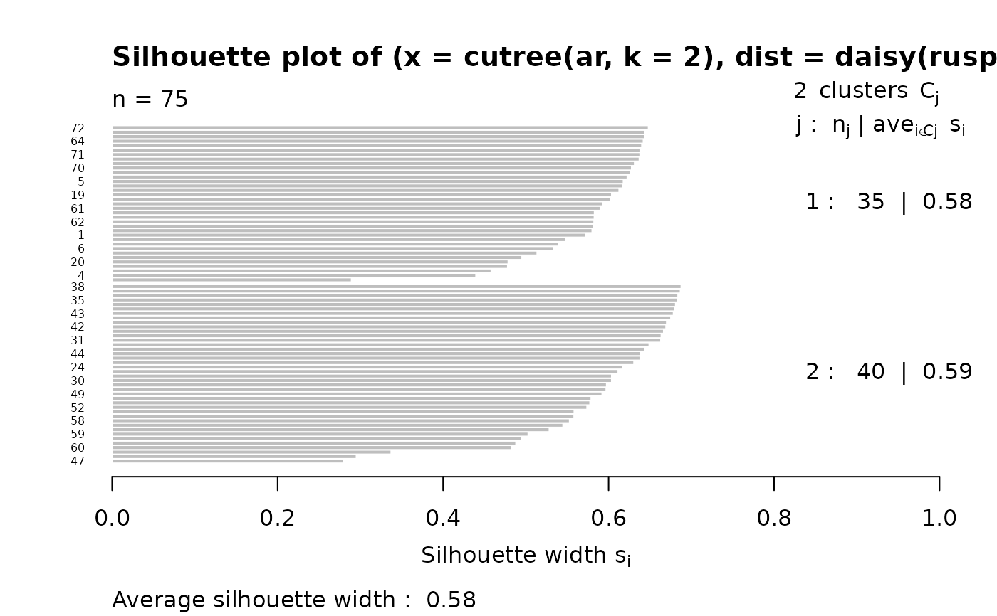
 ## 2 groups: Agnes() wasn't too good:
si4 <- silhouette(cutree(ar, k = 2), daisy(ruspini))
plot(si4, nmax = 80, cex.names = 0.5)
## 2 groups: Agnes() wasn't too good:
si4 <- silhouette(cutree(ar, k = 2), daisy(ruspini))
plot(si4, nmax = 80, cex.names = 0.5)