DIvisive ANAlysis Clustering

Computes a divisive hierarchical clustering of the dataset returning an object of class diana.

diana(x, diss = inherits(x, "dist"), metric = "euclidean", stand = FALSE,
      stop.at.k = FALSE,
      keep.diss = n < 100, keep.data = !diss, trace.lev = 0)

Arguments

x

data matrix or data frame, or dissimilarity matrix or object, depending on the value of the diss argument.

In case of a matrix or data frame, each row corresponds to an observation, and each column corresponds to a variable. All variables must be numeric. Missing values (NAs) are allowed.

In case of a dissimilarity matrix, x is typically the output of daisy or dist. Also a vector of length n*(n-1)/2 is allowed (where n is the number of observations), and will be interpreted in the same way as the output of the above-mentioned functions. Missing values (NAs) are not allowed.

diss

logical flag: if TRUE (default for dist or dissimilarity objects), then x will be considered as a dissimilarity matrix. If FALSE, then x will be considered as a matrix of observations by variables.

metric

character string specifying the metric to be used for calculating dissimilarities between observations.
The currently available options are "euclidean" and "manhattan". Euclidean distances are root sum-of-squares of differences, and manhattan distances are the sum of absolute differences. If x is already a dissimilarity matrix, then this argument will be ignored.

stand

logical; if true, the measurements in x are standardized before calculating the dissimilarities. Measurements are standardized for each variable (column), by subtracting the variable's mean value and dividing by the variable's mean absolute deviation. If x is already a dissimilarity matrix, then this argument will be ignored.

stop.at.k

logical or integer, FALSE by default. Otherwise must be integer, say \(k\), in \(\{1,2,..,n\}\), specifying that the diana algorithm should stop early. Non-default NOT YET IMPLEMENTED.

keep.diss, keep.data

logicals indicating if the dissimilarities and/or input data x should be kept in the result. Setting these to FALSE can give much smaller results and hence even save memory allocation time.

trace.lev

integer specifying a trace level for printing diagnostics during the algorithm. Default 0 does not print anything; higher values print increasingly more.

Value

an object of class "diana" representing the clustering; this class has methods for the following generic functions: print, summary, plot.

Further, the class "diana" inherits from "twins". Therefore, the generic function pltree can be used on a diana object, and as.hclust and as.dendrogram methods are available.

A legitimate diana object is a list with the following components:

order: a vector giving a permutation of the original observations to allow for plotting, in the sense that the branches of a clustering tree will not cross.
order.lab: a vector similar to order, but containing observation labels instead of observation numbers. This component is only available if the original observations were labelled.
height: a vector with the diameters of the clusters prior to splitting.
dc: the divisive coefficient, measuring the clustering structure of the dataset. For each observation i, denote by \(d(i)\) the diameter of the last cluster to which it belongs (before being split off as a single observation), divided by the diameter of the whole dataset. The dc is the average of all \(1 - d(i)\). It can also be seen as the average width (or the percentage filled) of the banner plot. Because dc grows with the number of observations, this measure should not be used to compare datasets of very different sizes.
merge: an (n-1) by 2 matrix, where n is the number of observations. Row i of merge describes the split at step n-i of the clustering. If a number \(j\) in row r is negative, then the single observation \(|j|\) is split off at stage n-r. If j is positive, then the cluster that will be splitted at stage n-j (described by row j), is split off at stage n-r.
diss: an object of class "dissimilarity", representing the total dissimilarity matrix of the dataset.
data: a matrix containing the original or standardized measurements, depending on the stand option of the function agnes. If a dissimilarity matrix was given as input structure, then this component is not available.

Details

diana is fully described in chapter 6 of Kaufman and Rousseeuw (1990). It is probably unique in computing a divisive hierarchy, whereas most other software for hierarchical clustering is agglomerative. Moreover, diana provides (a) the divisive coefficient (see diana.object) which measures the amount of clustering structure found; and (b) the banner, a novel graphical display (see plot.diana).

The diana-algorithm constructs a hierarchy of clusterings, starting with one large cluster containing all n observations. Clusters are divided until each cluster contains only a single observation.
At each stage, the cluster with the largest diameter is selected. (The diameter of a cluster is the largest dissimilarity between any two of its observations.)
To divide the selected cluster, the algorithm first looks for its most disparate observation (i.e., which has the largest average dissimilarity to the other observations of the selected cluster). This observation initiates the "splinter group". In subsequent steps, the algorithm reassigns observations that are closer to the "splinter group" than to the "old party". The result is a division of the selected cluster into two new clusters.

Examples

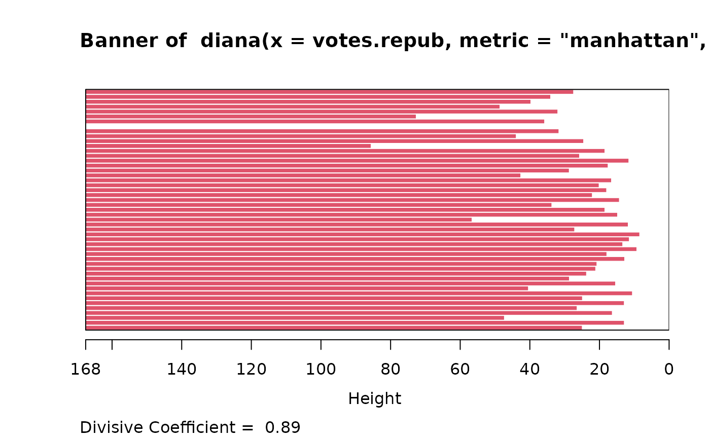
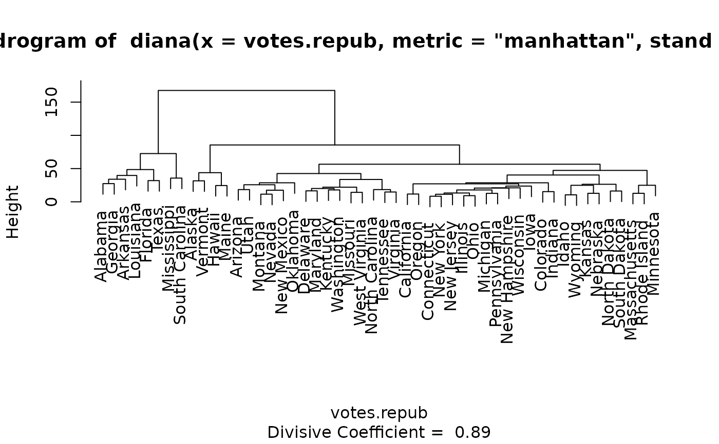
data(votes.repub)
dv <- diana(votes.repub, metric = "manhattan", stand = TRUE)
print(dv)
#> Merge:
#>       [,1] [,2]
#>  [1,]   -7  -32
#>  [2,]  -13  -35
#>  [3,]  -12  -50
#>  [4,]    1  -30
#>  [5,]  -26  -28
#>  [6,]   -5  -37
#>  [7,]  -22  -38
#>  [8,]  -21  -39
#>  [9,]  -16  -27
#> [10,]    4    2
#> [11,]  -25  -48
#> [12,]  -42  -46
#> [13,]   -6  -14
#> [14,]  -34  -41
#> [15,]   -8  -20
#> [16,]    5  -31
#> [17,]   10    7
#> [18,]  -17  -47
#> [19,]   -3  -44
#> [20,]  -33   12
#> [21,]   15   18
#> [22,]   17  -29
#> [23,]   22  -49
#> [24,]   21   11
#> [25,]   23  -15
#> [26,]  -11  -19
#> [27,]    3    9
#> [28,]    8  -23
#> [29,]   19   16
#> [30,]   27   14
#> [31,]    6   25
#> [32,]   -1  -10
#> [33,]   31   13
#> [34,]   29  -36
#> [35,]   -2  -45
#> [36,]   -9  -43
#> [37,]   24   20
#> [38,]   32   -4
#> [39,]  -24  -40
#> [40,]   38  -18
#> [41,]   33   30
#> [42,]   34   37
#> [43,]   35   26
#> [44,]   41   28
#> [45,]   40   36
#> [46,]   42   44
#> [47,]   45   39
#> [48,]   43   46
#> [49,]   47   48
#> Order of objects:
#>  [1] Alabama        Georgia        Arkansas       Louisiana      Florida       
#>  [6] Texas          Mississippi    South Carolina Alaska         Vermont       
#> [11] Hawaii         Maine          Arizona        Utah           Montana       
#> [16] Nevada         New Mexico     Oklahoma       Delaware       Maryland      
#> [21] Kentucky       Washington     Missouri       West Virginia  North Carolina
#> [26] Tennessee      Virginia       California     Oregon         Connecticut   
#> [31] New York       New Jersey     Illinois       Ohio           Michigan      
#> [36] Pennsylvania   New Hampshire  Wisconsin      Iowa           Colorado      
#> [41] Indiana        Idaho          Wyoming        Kansas         Nebraska      
#> [46] North Dakota   South Dakota   Massachusetts  Rhode Island   Minnesota     
#> Height:
#>  [1]  27.363453  33.969252  39.658259  48.534276  31.899654  72.598496
#>  [7]  35.691518 167.580197  31.582223  43.846009  24.487963  85.552482
#> [13]  18.393392  25.676314  11.493967  17.455521  28.625502  42.544800
#> [19]  16.485096  20.044499  17.875161  21.983729  14.218077  33.610713
#> [25]  18.397326  14.757619  56.556754  11.701321  27.058874   8.382005
#> [31]  11.368197  13.252375   9.230040  17.834836  12.708189  20.667139
#> [37]  21.039972  23.665856  28.605405  15.317027  40.339045  10.462936
#> [43]  24.835249  12.804188  26.362915  16.251922  47.257725  12.791603
#> [49]  24.872061
#> Divisive coefficient:
#> [1] 0.8869182
#> 
#> Available components:
#> [1] "order"     "height"    "dc"        "merge"     "diss"      "call"     
#> [7] "order.lab" "data"     
plot(dv) #-> plot.diana()  {w/ its own help + examples}



## Cut into 2 groups:
dv2 <- cutree(as.hclust(dv), k = 2)
table(dv2) # 8 and 42 group members
#> dv2
#>  1  2 
#>  8 42 
rownames(votes.repub)[dv2 == 1]
#> [1] "Alabama"        "Arkansas"       "Florida"        "Georgia"       
#> [5] "Louisiana"      "Mississippi"    "South Carolina" "Texas"         

## For two groups, does the metric matter ?
dv0 <- diana(votes.repub, stand = TRUE) # default: Euclidean
dv.2 <- cutree(as.hclust(dv0), k = 2)
table(dv2 == dv.2)## identical group assignments
#> 
#> TRUE 
#>   50 

str(as.dendrogram(dv0)) # {via as.dendrogram.twins() method}
#> --[dendrogram w/ 2 branches and 50 members at h = 31.1]
#>   |--[dendrogram w/ 2 branches and 8 members at h = 15.3]
#>   |  |--[dendrogram w/ 2 branches and 6 members at h = 10.5]
#>   |  |  |--[dendrogram w/ 2 branches and 3 members at h = 8.46]
#>   |  |  |  |--[dendrogram w/ 2 branches and 2 members at h = 6.28]
#>   |  |  |  |  |--leaf "Alabama" 
#>   |  |  |  |  `--leaf "Georgia" 
#>   |  |  |  `--leaf "Louisiana" 
#>   |  |  `--[dendrogram w/ 2 branches and 3 members at h = 7.68]
#>   |  |     |--[dendrogram w/ 2 branches and 2 members at h = 7.1]
#>   |  |     |  |--leaf "Arkansas" 
#>   |  |     |  `--leaf "Florida" 
#>   |  |     `--leaf "Texas" 
#>   |  `--[dendrogram w/ 2 branches and 2 members at h = 9.55]
#>   |     |--leaf "Mississippi" 
#>   |     `--leaf "South Carolina" 
#>   `--[dendrogram w/ 2 branches and 42 members at h = 17]
#>      |--[dendrogram w/ 2 branches and 4 members at h = 9.43]
#>      |  |--[dendrogram w/ 2 branches and 2 members at h = 6.45]
#>      |  |  |--leaf "Alaska" 
#>      |  |  `--leaf "Vermont" 
#>      |  `--[dendrogram w/ 2 branches and 2 members at h = 5.23]
#>      |     |--leaf "Hawaii" 
#>      |     `--leaf "Maine" 
#>      `--[dendrogram w/ 2 branches and 38 members at h = 12.5]
#>         |--[dendrogram w/ 2 branches and 9 members at h = 7.98]
#>         |  |--[dendrogram w/ 2 branches and 7 members at h = 6.12]
#>         |  |  |--[dendrogram w/ 2 branches and 4 members at h = 5.03]
#>         |  |  |  |--leaf "Arizona" 
#>         |  |  |  `--[dendrogram w/ 2 branches and 3 members at h = 4.11]
#>         |  |  |     |--leaf "Colorado" 
#>         |  |  |     `--[dendrogram w/ 2 branches and 2 members at h = 3.11]
#>         |  |  |        |--leaf "Montana" 
#>         |  |  |        `--leaf "Nevada" 
#>         |  |  `--[dendrogram w/ 2 branches and 3 members at h = 3.77]
#>         |  |     |--[dendrogram w/ 2 branches and 2 members at h = 2.28]
#>         |  |     |  |--leaf "Idaho" 
#>         |  |     |  `--leaf "Wyoming" 
#>         |  |     `--leaf "Utah" 
#>         |  `--[dendrogram w/ 2 branches and 2 members at h = 3.06]
#>         |     |--leaf "Kansas" 
#>         |     `--leaf "Nebraska" 
#>         `--[dendrogram w/ 2 branches and 29 members at h = 12.5]
#>            |--[dendrogram w/ 2 branches and 3 members at h = 5.1]
#>            |  |--[dendrogram w/ 2 branches and 2 members at h = 4.49]
#>            |  |  |--leaf "Kentucky" 
#>            |  |  `--leaf "Virginia" 
#>            |  `--leaf "Oklahoma" 
#>            `--[dendrogram w/ 2 branches and 26 members at h = 10.4]
#>               |--[dendrogram w/ 2 branches and 18 members at h = 7.26]
#>               |  |--[dendrogram w/ 2 branches and 14 members at h = 6.79]
#>               |  |  |--[dendrogram w/ 2 branches and 3 members at h = 3.72]
#>               |  |  |  |--leaf "California" 
#>               |  |  |  `--[dendrogram w/ 2 branches and 2 members at h = 2.64]
#>               |  |  |     |--leaf "Oregon" 
#>               |  |  |     `--leaf "Washington" 
#>               |  |  `--[dendrogram w/ 2 branches and 11 members at h = 5.82]
#>               |  |     |--[dendrogram w/ 2 branches and 9 members at h = 4.93]
#>               |  |     |  |--[dendrogram w/ 2 branches and 7 members at h = 4.13]
#>               |  |     |  |  |--[dendrogram w/ 2 branches and 2 members at h = 2.97]
#>               |  |     |  |  |  |--leaf "Connecticut" 
#>               |  |     |  |  |  `--leaf "New Hampshire" 
#>               |  |     |  |  `--[dendrogram w/ 2 branches and 5 members at h = 3.8]
#>               |  |     |  |     |--[dendrogram w/ 2 branches and 3 members at h = 2.61]
#>               |  |     |  |     |  |--[dendrogram w/ 2 branches and 2 members at h = 2.28]
#>               |  |     |  |     |  |  |--leaf "Illinois" 
#>               |  |     |  |     |  |  `--leaf "New Jersey" 
#>               |  |     |  |     |  `--leaf "New York" 
#>               |  |     |  |     `--[dendrogram w/ 2 branches and 2 members at h = 2.53]
#>               |  |     |  |        |--leaf "Indiana" 
#>               |  |     |  |        `--leaf "Ohio" 
#>               |  |     |  `--[dendrogram w/ 2 branches and 2 members at h = 2.77]
#>               |  |     |     |--leaf "Michigan" 
#>               |  |     |     `--leaf "Pennsylvania" 
#>               |  |     `--[dendrogram w/ 2 branches and 2 members at h = 3.61]
#>               |  |        |--leaf "Delaware" 
#>               |  |        `--leaf "New Mexico" 
#>               |  `--[dendrogram w/ 2 branches and 4 members at h = 4.37]
#>               |     |--[dendrogram w/ 2 branches and 3 members at h = 3.92]
#>               |     |  |--[dendrogram w/ 2 branches and 2 members at h = 2.73]
#>               |     |  |  |--leaf "Iowa" 
#>               |     |  |  `--leaf "South Dakota" 
#>               |     |  `--leaf "North Dakota" 
#>               |     `--leaf "Wisconsin" 
#>               `--[dendrogram w/ 2 branches and 8 members at h = 10.4]
#>                  |--[dendrogram w/ 2 branches and 5 members at h = 6.21]
#>                  |  |--leaf "Maryland" 
#>                  |  `--[dendrogram w/ 2 branches and 4 members at h = 5.71]
#>                  |     |--[dendrogram w/ 2 branches and 2 members at h = 3.17]
#>                  |     |  |--leaf "Missouri" 
#>                  |     |  `--leaf "West Virginia" 
#>                  |     `--[dendrogram w/ 2 branches and 2 members at h = 3.7]
#>                  |        |--leaf "North Carolina" 
#>                  |        `--leaf "Tennessee" 
#>                  `--[dendrogram w/ 2 branches and 3 members at h = 5.53]
#>                     |--[dendrogram w/ 2 branches and 2 members at h = 3.21]
#>                     |  |--leaf "Massachusetts" 
#>                     |  `--leaf "Rhode Island" 
#>                     `--leaf "Minnesota" 

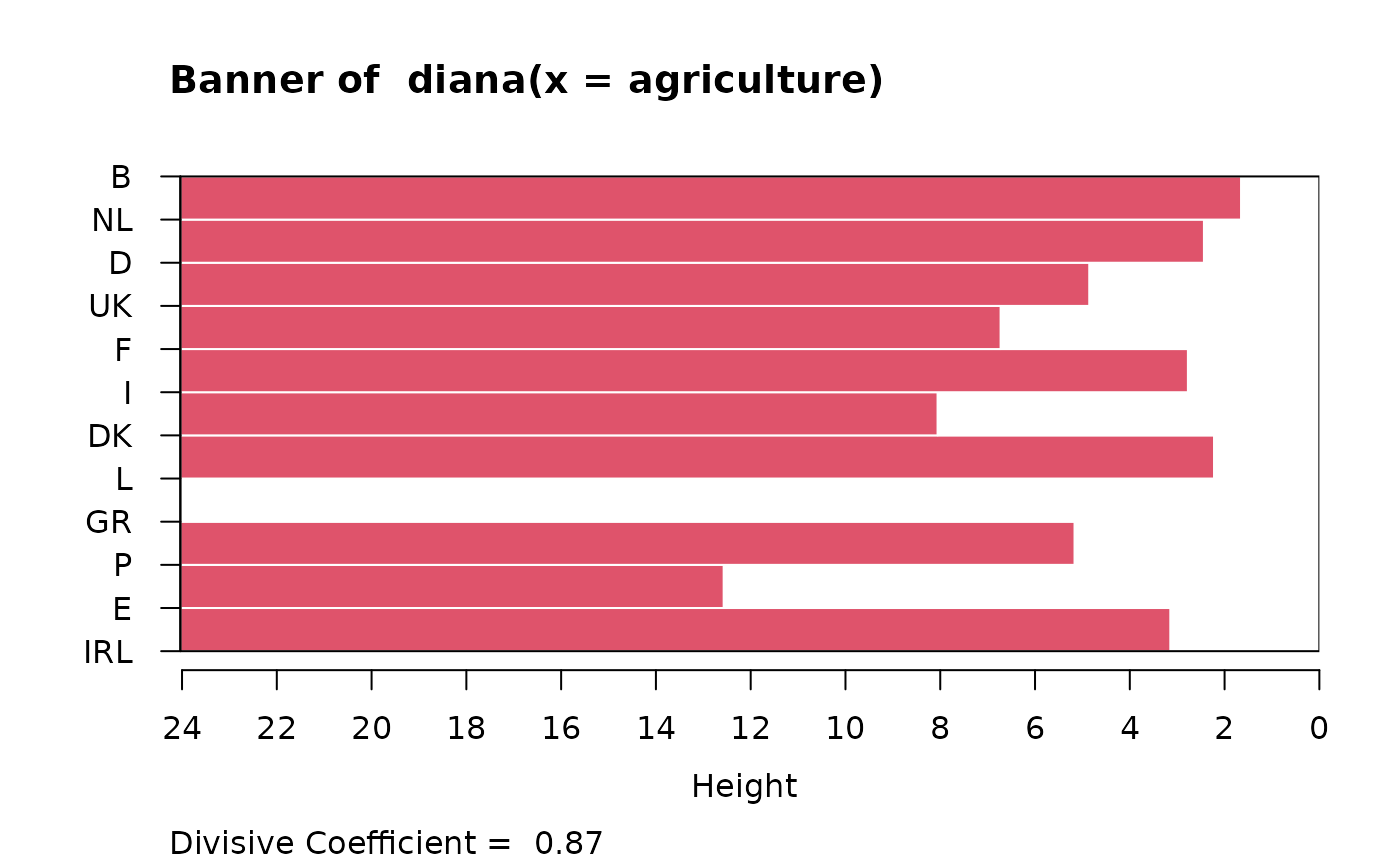
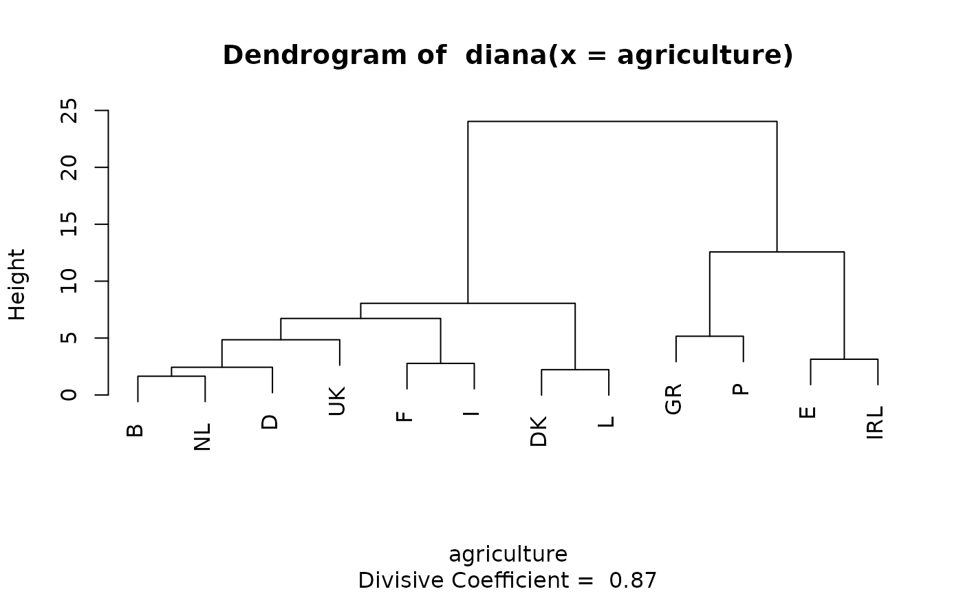
data(agriculture)
## Plot similar to Figure 8 in ref
if (FALSE) plot(diana(agriculture), ask = TRUE) # \dontrun{}

Arguments

Value

Details

See also

Examples