Attributes of Animals
animals.RdThis data set considers 6 binary attributes for 20 animals.
data(animals)Format
A data frame with 20 observations on 6 variables:
| [ , 1] | war | warm-blooded |
| [ , 2] | fly | can fly |
| [ , 3] | ver | vertebrate |
| [ , 4] | end | endangered |
| [ , 5] | gro | live in groups |
| [ , 6] | hai | have hair |
All variables are encoded as 1 = 'no', 2 = 'yes'.
Source
Leonard Kaufman and Peter J. Rousseeuw (1990): Finding Groups in Data (pp 297ff). New York: Wiley.
Details
This dataset is useful for illustrating monothetic (only a single variable is used for each split) hierarchical clustering.
References
see Struyf, Hubert & Rousseeuw (1996), in agnes.
Examples
data(animals)
apply(animals,2, table) # simple overview
#> war fly ver end gro hai
#> 1 10 16 6 12 6 11
#> 2 10 4 14 6 11 9
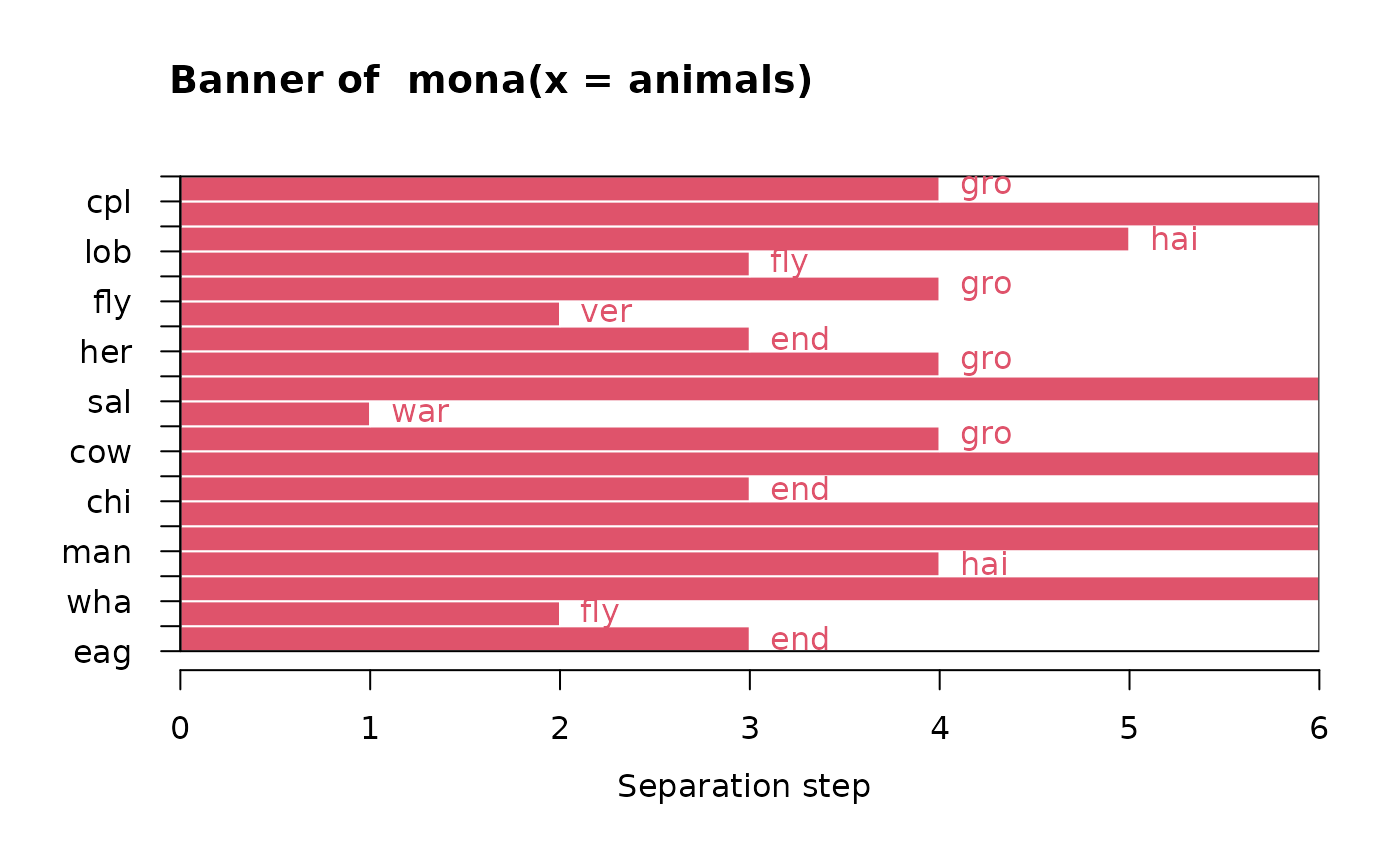
ma <- mona(animals)
ma
#> mona(x, ..) fit; x of dimension 20x6
#> Because of NA's, revised data:
#> war fly ver end gro hai
#> ant 0 0 0 0 1 0
#> bee 0 1 0 0 1 1
#> cat 1 0 1 0 0 1
#> cpl 0 0 0 0 0 1
#> chi 1 0 1 1 1 1
#> cow 1 0 1 0 1 1
#> duc 1 1 1 0 1 0
#> eag 1 1 1 1 0 0
#> ele 1 0 1 1 1 0
#> fly 0 1 0 0 0 0
#> fro 0 0 1 1 0 0
#> her 0 0 1 0 1 0
#> lio 1 0 1 1 1 1
#> liz 0 0 1 0 0 0
#> lob 0 0 0 0 0 0
#> man 1 0 1 1 1 1
#> rab 1 0 1 0 1 1
#> sal 0 0 1 0 0 0
#> spi 0 0 0 0 0 1
#> wha 1 0 1 1 1 0
#> Order of objects:
#> [1] ant cpl spi lob bee fly fro her liz sal cat cow rab chi lio man ele wha duc
#> [20] eag
#> Variable used:
#> [1] gro NULL hai fly gro ver end gro NULL war gro NULL end NULL NULL
#> [16] hai NULL fly end
#> Separation step:
#> [1] 4 0 5 3 4 2 3 4 0 1 4 0 3 0 0 4 0 2 3
#>
#> Available components:
#> [1] "data" "hasNA" "order" "variable" "step" "order.lab"
#> [7] "call"
## Plot similar to Figure 10 in Struyf et al (1996)
plot(ma)