Test Linear Hypothesis
linearHypothesis.RdGeneric function for testing a linear hypothesis, and methods
for linear models, generalized linear models, multivariate linear
models, linear and generalized linear mixed-effects models,
generalized linear models fit with svyglm in the survey package,
robust linear models fit with rlm in the MASS package,
and other models that have methods for coef and vcov.
For mixed-effects models, the tests are Wald chi-square tests for the fixed effects.
Usage
linearHypothesis(model, ...)

lht(model, ...)

# Default S3 method
linearHypothesis(model, hypothesis.matrix, rhs=NULL,
    test=c("Chisq", "F"), vcov.=NULL, singular.ok=FALSE, verbose=FALSE,
    coef. = coef(model), suppress.vcov.msg=FALSE, error.df, ...)

# S3 method for class 'lm'
linearHypothesis(model, hypothesis.matrix, rhs=NULL,
    test=c("F", "Chisq"), vcov.=NULL,
  white.adjust=c(FALSE, TRUE, "hc3", "hc0", "hc1", "hc2", "hc4"),
  singular.ok=FALSE, ...)

# S3 method for class 'glm'
linearHypothesis(model,  ...)

# S3 method for class 'lmList'
linearHypothesis(model,  ..., vcov.=vcov, coef.=coef)

# S3 method for class 'nlsList'
linearHypothesis(model,  ..., vcov.=vcov, coef.=coef)

# S3 method for class 'mlm'
linearHypothesis(model, hypothesis.matrix, rhs=NULL, SSPE, V,
    test, idata, icontrasts=c("contr.sum", "contr.poly"), idesign, iterms,
    check.imatrix=TRUE, P=NULL, title="", singular.ok=FALSE, verbose=FALSE, ...)

# S3 method for class 'polr'
linearHypothesis(model, hypothesis.matrix, rhs=NULL, vcov.,
  verbose=FALSE, ...)

# S3 method for class 'linearHypothesis.mlm'
print(x, SSP=TRUE, SSPE=SSP,
    digits=getOption("digits"), ...)

# S3 method for class 'lme'
linearHypothesis(model, hypothesis.matrix, rhs=NULL,
    vcov.=NULL, singular.ok=FALSE, verbose=FALSE, ...)

# S3 method for class 'mer'
linearHypothesis(model, hypothesis.matrix, rhs=NULL,
    vcov.=NULL, test=c("Chisq", "F"), singular.ok=FALSE, verbose=FALSE, ...)

# S3 method for class 'merMod'
linearHypothesis(model, hypothesis.matrix, rhs=NULL,
      vcov.=NULL, test=c("Chisq", "F"), singular.ok=FALSE, verbose=FALSE, ...)

# S3 method for class 'svyglm'
linearHypothesis(model, ...)

# S3 method for class 'rlm'
linearHypothesis(model, ...)

# S3 method for class 'survreg'
linearHypothesis(model, hypothesis.matrix, rhs=NULL,
    test=c("Chisq", "F"), vcov., verbose=FALSE, ...)

matchCoefs(model, pattern, ...)

# Default S3 method
matchCoefs(model, pattern, coef.=coef, ...)

# S3 method for class 'lme'
matchCoefs(model, pattern, ...)

# S3 method for class 'mer'
matchCoefs(model, pattern, ...)

# S3 method for class 'merMod'
matchCoefs(model, pattern, ...)

# S3 method for class 'mlm'
matchCoefs(model, pattern, ...)

# S3 method for class 'lmList'
matchCoefs(model, pattern, ...)
Arguments
- model
fitted model object. The default method of
linearHypothesisworks for models for which the estimated parameters can be retrieved bycoefand the corresponding estimated covariance matrix byvcov. See the Details for more information.- hypothesis.matrix
matrix (or vector) giving linear combinations of coefficients by rows, or a character vector giving the hypothesis in symbolic form (see Details).
- rhs
right-hand-side vector for hypothesis, with as many entries as rows in the hypothesis matrix; can be omitted, in which case it defaults to a vector of zeroes. For a multivariate linear model,
rhsis a matrix, defaulting to 0. This argument isn't available for F-tests for linear mixed models.- singular.ok
if
FALSE(the default), a model with aliased coefficients produces an error; ifTRUE, the aliased coefficients are ignored, and the hypothesis matrix should not have columns for them. For a multivariate linear model: will return the hypothesis and error SSP matrices even if the latter is singular; useful for computing univariate repeated-measures ANOVAs where there are fewer subjects than df for within-subject effects.- error.df
For the
defaultlinearHypothesismethod, if an F-test is requested and iferror.dfis missing, the error degrees of freedom will be computed by applying thedf.residualfunction to the model; ifdf.residualreturnsNULLorNA, then a chi-square test will be substituted for the F-test (with a message to that effect.- idata
an optional data frame giving a factor or factors defining the intra-subject model for multivariate repeated-measures data. See Details for an explanation of the intra-subject design and for further explanation of the other arguments relating to intra-subject factors.
- icontrasts
names of contrast-generating functions to be applied by default to factors and ordered factors, respectively, in the within-subject “data”; the contrasts must produce an intra-subject model matrix in which different terms are orthogonal.
- idesign
a one-sided model formula using the “data” in
idataand specifying the intra-subject design.- iterms
the quoted name of a term, or a vector of quoted names of terms, in the intra-subject design to be tested.
- check.imatrix
check that columns of the intra-subject model matrix for different terms are mutually orthogonal (default,
TRUE). Set toFALSEonly if you have already checked that the intra-subject model matrix is block-orthogonal.- P
transformation matrix to be applied to the repeated measures in multivariate repeated-measures data; if
NULLand no intra-subject model is specified, no response-transformation is applied; if an intra-subject model is specified via theidata,idesign, and (optionally)icontrastsarguments, thenPis generated automatically from theitermsargument.- SSPE
in
linearHypothesismethod formlmobjects: optional error sum-of-squares-and-products matrix; if missing, it is computed from the model. Inprintmethod forlinearHypothesis.mlmobjects: ifTRUE, print the sum-of-squares and cross-products matrix for error.- test
character string,
"F"or"Chisq", specifying whether to compute the finite-sample F statistic (with approximate F distribution) or the large-sample Chi-squared statistic (with asymptotic Chi-squared distribution). For a multivariate linear model, the multivariate test statistic to report — one or more of"Pillai","Wilks","Hotelling-Lawley", or"Roy", with"Pillai"as the default.- title
an optional character string to label the output.
- V
inverse of sum of squares and products of the model matrix; if missing it is computed from the model.
- vcov.
a function for estimating the covariance matrix of the regression coefficients, e.g.,
hccm, or an estimated covariance matrix formodel. See alsowhite.adjust. For the"lmList"and"nlsList"methods,vcov.must be a function (defaulting tovcov) to be applied to each model in the list.Note that arguments supplied to
...are not passed tovcov.when it's a function; in this case either use an anonymous function in which the additional arguments are set, or supply the coefficient covariance matrix directly (see the examples).- coef.
a vector of coefficient estimates. The default is to get the coefficient estimates from the
modelargument, but the user can input any vector of the correct length. For the"lmList"and"nlsList"methods,coef.must be a function (defaulting tocoef) to be applied to each model in the list.- white.adjust
logical or character. Convenience interface to
hccm(instead of using the argumentvcov.). Can be set either to a character value specifying thetypeargument ofhccmorTRUE, in which case"hc3"is used implicitly. The default isFALSE.- verbose
If
TRUE, the hypothesis matrix, right-hand-side vector (or matrix), and estimated value of the hypothesis are printed to standard output; ifFALSE(the default), the hypothesis is only printed in symbolic form and the value of the hypothesis is not printed.- x
an object produced by
linearHypothesis.mlm.- SSP
if
TRUE(the default), print the sum-of-squares and cross-products matrix for the hypothesis and the response-transformation matrix.- digits
minimum number of signficiant digits to print.
- pattern
a regular expression to be matched against coefficient names.
- suppress.vcov.msg
for internal use by methods that call the default method.
- ...
arguments to pass down.
Details
linearHypothesis computes either a finite-sample F statistic or asymptotic Chi-squared
statistic for carrying out a Wald-test-based comparison between a model
and a linearly restricted model. The default method will work with any
model object for which the coefficient vector can be retrieved by
coef and the coefficient-covariance matrix by vcov (otherwise
the argument vcov. has to be set explicitly). For computing the
F statistic (but not the Chi-squared statistic) a df.residual
method needs to be available. If a formula method exists, it is
used for pretty printing.
The method for "lm" objects calls the default method, but it
changes the default test to "F", supports the convenience argument
white.adjust (for backwards compatibility), and enhances the output
by the residual sums of squares. For "glm" objects just the default
method is called (bypassing the "lm" method). The "svyglm" method
also calls the default method.
Multinomial logit models fit by the multinom function in the nnet package invoke the default method, and the coefficient names are composed from the response-level names and conventional coefficient names, separated by a period ("."): see one of the examples below.
The function lht also dispatches to linearHypothesis.
The hypothesis matrix can be supplied as a numeric matrix (or vector), the rows of which specify linear combinations of the model coefficients, which are tested equal to the corresponding entries in the right-hand-side vector, which defaults to a vector of zeroes.
Alternatively, the hypothesis can be specified symbolically as a character vector with one or more elements, each of which gives either a linear combination of coefficients, or a linear equation in the coefficients (i.e., with both a left and right side separated by an equals sign). Components of a linear expression or linear equation can consist of numeric constants, or numeric constants multiplying coefficient names (in which case the number precedes the coefficient, and may be separated from it by spaces or an asterisk); constants of 1 or -1 may be omitted. Spaces are always optional. Components are separated by plus or minus signs. Newlines or tabs in hypotheses will be treated as spaces. See the examples below.
If the user sets the arguments coef. and vcov., then the computations
are done without reference to the model argument. This is like assuming
that coef. is normally distibuted with estimated variance vcov.
and the linearHypothesis will compute tests on the mean vector for
coef., without actually using the model argument.
A linear hypothesis for a multivariate linear model (i.e., an object of
class "mlm") can optionally include an intra-subject transformation matrix
for a repeated-measures design.
If the intra-subject transformation is absent (the default), the multivariate
test concerns all of the corresponding coefficients for the response variables.
There are two ways to specify the transformation matrix for the
repeated measures:
The transformation matrix can be specified directly via the
Pargument.A data frame can be provided defining the repeated-measures factor or factors via
idata, with default contrasts given by theicontrastsargument. An intra-subject model-matrix is generated from the one-sided formula specified by theidesignargument; columns of the model matrix corresponding to different terms in the intra-subject model must be orthogonal (as is insured by the default contrasts). Note that the contrasts given inicontrastscan be overridden by assigning specific contrasts to the factors inidata. The repeated-measures transformation matrix consists of the columns of the intra-subject model matrix corresponding to the term or terms initerms. In most instances, this will be the simpler approach, and indeed, most tests of interests can be generated automatically via theAnovafunction.
matchCoefs is a convenience function that can sometimes help in formulating hypotheses; for example
matchCoefs(mod, ":") will return the names of all interaction coefficients in the model mod.
Value
For a univariate model, an object of class "anova"
which contains the residual degrees of freedom
in the model, the difference in degrees of freedom, Wald statistic
(either "F" or "Chisq"), and corresponding p value.
The value of the linear hypothesis and its covariance matrix are returned
respectively as "value" and "vcov" attributes of the object
(but not printed).
For a multivariate linear model, an object of class
"linearHypothesis.mlm", which contains sums-of-squares-and-product
matrices for the hypothesis and for error, degrees of freedom for the
hypothesis and error, and some other information.
The returned object normally would be printed.
References
Fox, J. (2016) Applied Regression Analysis and Generalized Linear Models, Third Edition. Sage.
Fox, J. and Weisberg, S. (2019) An R Companion to Applied Regression, Third Edition, Sage.
Hand, D. J., and Taylor, C. C. (1987) Multivariate Analysis of Variance and Repeated Measures: A Practical Approach for Behavioural Scientists. Chapman and Hall.
O'Brien, R. G., and Kaiser, M. K. (1985) MANOVA method for analyzing repeated measures designs: An extensive primer. Psychological Bulletin 97, 316–333.
Author
Achim Zeileis and John Fox jfox@mcmaster.ca
Examples
mod.davis <- lm(weight ~ repwt, data=Davis)
## the following are equivalent:
linearHypothesis(mod.davis, diag(2), c(0,1))
#>
#> Linear hypothesis test:
#> (Intercept) = 0
#> repwt = 1
#>
#> Model 1: restricted model
#> Model 2: weight ~ repwt
#>
#> Res.Df RSS Df Sum of Sq F Pr(>F)
#> 1 183 13074
#> 2 181 12828 2 245.97 1.7353 0.1793
linearHypothesis(mod.davis, c("(Intercept) = 0", "repwt = 1"))
#>
#> Linear hypothesis test:
#> (Intercept) = 0
#> repwt = 1
#>
#> Model 1: restricted model
#> Model 2: weight ~ repwt
#>
#> Res.Df RSS Df Sum of Sq F Pr(>F)
#> 1 183 13074
#> 2 181 12828 2 245.97 1.7353 0.1793
linearHypothesis(mod.davis, c("(Intercept)", "repwt"), c(0,1))
#>
#> Linear hypothesis test:
#> (Intercept) = 0
#> repwt = 1
#>
#> Model 1: restricted model
#> Model 2: weight ~ repwt
#>
#> Res.Df RSS Df Sum of Sq F Pr(>F)
#> 1 183 13074
#> 2 181 12828 2 245.97 1.7353 0.1793
linearHypothesis(mod.davis, c("(Intercept)", "repwt = 1"))
#>
#> Linear hypothesis test:
#> (Intercept) = 0
#> repwt = 1
#>
#> Model 1: restricted model
#> Model 2: weight ~ repwt
#>
#> Res.Df RSS Df Sum of Sq F Pr(>F)
#> 1 183 13074
#> 2 181 12828 2 245.97 1.7353 0.1793
## use asymptotic Chi-squared statistic
linearHypothesis(mod.davis, c("(Intercept) = 0", "repwt = 1"), test = "Chisq")
#>
#> Linear hypothesis test:
#> (Intercept) = 0
#> repwt = 1
#>
#> Model 1: restricted model
#> Model 2: weight ~ repwt
#>
#> Res.Df RSS Df Sum of Sq Chisq Pr(>Chisq)
#> 1 183 13074
#> 2 181 12828 2 245.97 3.4706 0.1763
## the following are equivalent:
## use HC3 standard errors via white.adjust option
linearHypothesis(mod.davis, c("(Intercept) = 0", "repwt = 1"),
white.adjust = TRUE)
#>
#> Linear hypothesis test:
#> (Intercept) = 0
#> repwt = 1
#>
#> Model 1: restricted model
#> Model 2: weight ~ repwt
#>
#> Note: Coefficient covariance matrix supplied.
#>
#> Res.Df Df F Pr(>F)
#> 1 183
#> 2 181 2 3.3896 0.03588 *
#> ---
#> Signif. codes: 0 ‘***’ 0.001 ‘**’ 0.01 ‘*’ 0.05 ‘.’ 0.1 ‘ ’ 1
## covariance matrix *function* (where type = "hc3" is the default)
linearHypothesis(mod.davis, c("(Intercept) = 0", "repwt = 1"), vcov. = hccm)
#>
#> Linear hypothesis test:
#> (Intercept) = 0
#> repwt = 1
#>
#> Model 1: restricted model
#> Model 2: weight ~ repwt
#>
#> Note: Coefficient covariance matrix supplied.
#>
#> Res.Df Df F Pr(>F)
#> 1 183
#> 2 181 2 3.3896 0.03588 *
#> ---
#> Signif. codes: 0 ‘***’ 0.001 ‘**’ 0.01 ‘*’ 0.05 ‘.’ 0.1 ‘ ’ 1
## covariance matrix *estimate*, specifying type explicitly
linearHypothesis(mod.davis, c("(Intercept) = 0", "repwt = 1"),
vcov = hccm(mod.davis, type = "hc3"))
#>
#> Linear hypothesis test:
#> (Intercept) = 0
#> repwt = 1
#>
#> Model 1: restricted model
#> Model 2: weight ~ repwt
#>
#> Note: Coefficient covariance matrix supplied.
#>
#> Res.Df Df F Pr(>F)
#> 1 183
#> 2 181 2 3.3896 0.03588 *
#> ---
#> Signif. codes: 0 ‘***’ 0.001 ‘**’ 0.01 ‘*’ 0.05 ‘.’ 0.1 ‘ ’ 1
## specifying additional type argument to covariance matrix function
linearHypothesis(mod.davis, c("(Intercept) = 0", "repwt = 1"),
vcov = function(m) hccm(m, type = "hc3"))
#>
#> Linear hypothesis test:
#> (Intercept) = 0
#> repwt = 1
#>
#> Model 1: restricted model
#> Model 2: weight ~ repwt
#>
#> Note: Coefficient covariance matrix supplied.
#>
#> Res.Df Df F Pr(>F)
#> 1 183
#> 2 181 2 3.3896 0.03588 *
#> ---
#> Signif. codes: 0 ‘***’ 0.001 ‘**’ 0.01 ‘*’ 0.05 ‘.’ 0.1 ‘ ’ 1
mod.duncan <- lm(prestige ~ income + education, data=Duncan)
## the following are all equivalent:
linearHypothesis(mod.duncan, "1*income - 1*education = 0")
#>
#> Linear hypothesis test:
#> income - education = 0
#>
#> Model 1: restricted model
#> Model 2: prestige ~ income + education
#>
#> Res.Df RSS Df Sum of Sq F Pr(>F)
#> 1 43 7518.9
#> 2 42 7506.7 1 12.195 0.0682 0.7952
linearHypothesis(mod.duncan, "income = education")
#>
#> Linear hypothesis test:
#> income - education = 0
#>
#> Model 1: restricted model
#> Model 2: prestige ~ income + education
#>
#> Res.Df RSS Df Sum of Sq F Pr(>F)
#> 1 43 7518.9
#> 2 42 7506.7 1 12.195 0.0682 0.7952
linearHypothesis(mod.duncan, "income - education")
#>
#> Linear hypothesis test:
#> income - education = 0
#>
#> Model 1: restricted model
#> Model 2: prestige ~ income + education
#>
#> Res.Df RSS Df Sum of Sq F Pr(>F)
#> 1 43 7518.9
#> 2 42 7506.7 1 12.195 0.0682 0.7952
linearHypothesis(mod.duncan, "1income - 1education = 0")
#>
#> Linear hypothesis test:
#> income - education = 0
#>
#> Model 1: restricted model
#> Model 2: prestige ~ income + education
#>
#> Res.Df RSS Df Sum of Sq F Pr(>F)
#> 1 43 7518.9
#> 2 42 7506.7 1 12.195 0.0682 0.7952
linearHypothesis(mod.duncan, "0 = 1*income - 1*education")
#>
#> Linear hypothesis test:
#> - income + education = 0
#>
#> Model 1: restricted model
#> Model 2: prestige ~ income + education
#>
#> Res.Df RSS Df Sum of Sq F Pr(>F)
#> 1 43 7518.9
#> 2 42 7506.7 1 12.195 0.0682 0.7952
linearHypothesis(mod.duncan, "income-education=0")
#>
#> Linear hypothesis test:
#> income - education = 0
#>
#> Model 1: restricted model
#> Model 2: prestige ~ income + education
#>
#> Res.Df RSS Df Sum of Sq F Pr(>F)
#> 1 43 7518.9
#> 2 42 7506.7 1 12.195 0.0682 0.7952
linearHypothesis(mod.duncan, "1*income - 1*education + 1 = 1")
#>
#> Linear hypothesis test:
#> income - education = 0
#>
#> Model 1: restricted model
#> Model 2: prestige ~ income + education
#>
#> Res.Df RSS Df Sum of Sq F Pr(>F)
#> 1 43 7518.9
#> 2 42 7506.7 1 12.195 0.0682 0.7952
linearHypothesis(mod.duncan, "2income = 2*education")
#>
#> Linear hypothesis test:
#> 2 income - 2 education = 0
#>
#> Model 1: restricted model
#> Model 2: prestige ~ income + education
#>
#> Res.Df RSS Df Sum of Sq F Pr(>F)
#> 1 43 7518.9
#> 2 42 7506.7 1 12.195 0.0682 0.7952
mod.duncan.2 <- lm(prestige ~ type*(income + education), data=Duncan)
coefs <- names(coef(mod.duncan.2))
## test against the null model (i.e., only the intercept is not set to 0)
linearHypothesis(mod.duncan.2, coefs[-1])
#>
#> Linear hypothesis test:
#> typeprof = 0
#> typewc = 0
#> income = 0
#> education = 0
#> typeprof:income = 0
#> typewc:income = 0
#> typeprof:education = 0
#> typewc:education = 0
#>
#> Model 1: restricted model
#> Model 2: prestige ~ type * (income + education)
#>
#> Res.Df RSS Df Sum of Sq F Pr(>F)
#> 1 44 43688
#> 2 36 3351 8 40337 54.174 < 2.2e-16 ***
#> ---
#> Signif. codes: 0 ‘***’ 0.001 ‘**’ 0.01 ‘*’ 0.05 ‘.’ 0.1 ‘ ’ 1
## test all interaction coefficients equal to 0
linearHypothesis(mod.duncan.2, coefs[grep(":", coefs)], verbose=TRUE)
#>
#> Hypothesis matrix:
#> (Intercept) typeprof typewc income education typeprof:income
#> typeprof:income 0 0 0 0 0 1
#> typewc:income 0 0 0 0 0 0
#> typeprof:education 0 0 0 0 0 0
#> typewc:education 0 0 0 0 0 0
#> typewc:income typeprof:education typewc:education
#> typeprof:income 0 0 0
#> typewc:income 1 0 0
#> typeprof:education 0 1 0
#> typewc:education 0 0 1
#>
#> Right-hand-side vector:
#> [1] 0 0 0 0
#>
#> Estimated linear function (hypothesis.matrix %*% coef - rhs)
#> typeprof:income typewc:income typeprof:education typewc:education
#> -0.36914256 -0.36030837 0.01859107 0.10677092
#>
#>
#> Estimated variance/covariance matrix for linear function
#> typeprof:income typewc:income typeprof:education
#> typeprof:income 0.04156710 0.017091995 -0.02462562
#> typewc:income 0.01709200 0.067378054 -0.01508772
#> typeprof:education -0.02462562 -0.015087722 0.10135862
#> typewc:education -0.01508772 -0.009442361 0.07828368
#> typewc:education
#> typeprof:income -0.015087722
#> typewc:income -0.009442361
#> typeprof:education 0.078283679
#> typewc:education 0.131161899
#>
#>
#> Linear hypothesis test:
#> typeprof:income = 0
#> typewc:income = 0
#> typeprof:education = 0
#> typewc:education = 0
#>
#> Model 1: restricted model
#> Model 2: prestige ~ type * (income + education)
#>
#> Res.Df RSS Df Sum of Sq F Pr(>F)
#> 1 40 3798.0
#> 2 36 3350.6 4 447.31 1.2015 0.327
linearHypothesis(mod.duncan.2, matchCoefs(mod.duncan.2, ":"), verbose=TRUE) # equivalent
#>
#> Hypothesis matrix:
#> (Intercept) typeprof typewc income education typeprof:income
#> typeprof:income 0 0 0 0 0 1
#> typewc:income 0 0 0 0 0 0
#> typeprof:education 0 0 0 0 0 0
#> typewc:education 0 0 0 0 0 0
#> typewc:income typeprof:education typewc:education
#> typeprof:income 0 0 0
#> typewc:income 1 0 0
#> typeprof:education 0 1 0
#> typewc:education 0 0 1
#>
#> Right-hand-side vector:
#> [1] 0 0 0 0
#>
#> Estimated linear function (hypothesis.matrix %*% coef - rhs)
#> typeprof:income typewc:income typeprof:education typewc:education
#> -0.36914256 -0.36030837 0.01859107 0.10677092
#>
#>
#> Estimated variance/covariance matrix for linear function
#> typeprof:income typewc:income typeprof:education
#> typeprof:income 0.04156710 0.017091995 -0.02462562
#> typewc:income 0.01709200 0.067378054 -0.01508772
#> typeprof:education -0.02462562 -0.015087722 0.10135862
#> typewc:education -0.01508772 -0.009442361 0.07828368
#> typewc:education
#> typeprof:income -0.015087722
#> typewc:income -0.009442361
#> typeprof:education 0.078283679
#> typewc:education 0.131161899
#>
#>
#> Linear hypothesis test:
#> typeprof:income = 0
#> typewc:income = 0
#> typeprof:education = 0
#> typewc:education = 0
#>
#> Model 1: restricted model
#> Model 2: prestige ~ type * (income + education)
#>
#> Res.Df RSS Df Sum of Sq F Pr(>F)
#> 1 40 3798.0
#> 2 36 3350.6 4 447.31 1.2015 0.327
lh <- linearHypothesis(mod.duncan.2, coefs[grep(":", coefs)])
attr(lh, "value") # value of linear function
#> [,1]
#> typeprof:income -0.36914256
#> typewc:income -0.36030837
#> typeprof:education 0.01859107
#> typewc:education 0.10677092
attr(lh, "vcov") # covariance matrix of linear function
#> typeprof:income typewc:income typeprof:education
#> typeprof:income 0.04156710 0.017091995 -0.02462562
#> typewc:income 0.01709200 0.067378054 -0.01508772
#> typeprof:education -0.02462562 -0.015087722 0.10135862
#> typewc:education -0.01508772 -0.009442361 0.07828368
#> typewc:education
#> typeprof:income -0.015087722
#> typewc:income -0.009442361
#> typeprof:education 0.078283679
#> typewc:education 0.131161899
## a multivariate linear model for repeated-measures data
## see ?OBrienKaiser for a description of the data set used in this example.
mod.ok <- lm(cbind(pre.1, pre.2, pre.3, pre.4, pre.5,
post.1, post.2, post.3, post.4, post.5,
fup.1, fup.2, fup.3, fup.4, fup.5) ~ treatment*gender,
data=OBrienKaiser)
coef(mod.ok)
#> pre.1 pre.2 pre.3 pre.4 pre.5
#> (Intercept) 3.9027778 4.2777778 5.43055556 4.6111111 4.1388889
#> treatment1 0.1180556 0.1388889 -0.07638889 0.1805556 0.1944444
#> treatment2 -0.2291667 -0.3333333 -0.14583333 -0.7083333 -0.6666667
#> gender1 -0.6527778 -0.7777778 -0.18055556 -0.1111111 -0.6388889
#> treatment1:gender1 -0.4930556 -0.3888889 -0.54861111 -0.1805556 -0.1944444
#> treatment2:gender1 0.6041667 0.5833333 0.27083333 0.7083333 1.1666667
#> post.1 post.2 post.3 post.4 post.5
#> (Intercept) 5.0277778 5.5416667 6.9166667 6.36111111 4.833333e+00
#> treatment1 0.7638889 0.8958333 0.8333333 0.72222222 9.166667e-01
#> treatment2 0.2916667 0.1875000 -0.2500000 0.08333333 -1.233135e-16
#> gender1 -0.8611111 -0.4583333 -0.4166667 -0.52777778 -1.000000e+00
#> treatment1:gender1 -0.6805556 -0.6041667 -0.3333333 -0.55555556 -5.000000e-01
#> treatment2:gender1 0.9583333 0.6875000 0.2500000 0.91666667 1.250000e+00
#> fup.1 fup.2 fup.3 fup.4 fup.5
#> (Intercept) 6.0138889 6.1527778 7.7777778 6.16666667 5.3472222
#> treatment1 0.9236111 1.0347222 1.0972222 0.95833333 0.8819444
#> treatment2 -0.0625000 -0.0625000 -0.1250000 0.12500000 0.2291667
#> gender1 -0.5972222 -0.9027778 -0.7777778 -0.83333333 -0.4305556
#> treatment1:gender1 -0.2152778 -0.1597222 -0.3472222 -0.04166667 -0.1736111
#> treatment2:gender1 0.6875000 1.1875000 0.8750000 1.12500000 0.3958333
## specify the model for the repeated measures:
phase <- factor(rep(c("pretest", "posttest", "followup"), c(5, 5, 5)),
levels=c("pretest", "posttest", "followup"))
hour <- ordered(rep(1:5, 3))
idata <- data.frame(phase, hour)
idata
#> phase hour
#> 1 pretest 1
#> 2 pretest 2
#> 3 pretest 3
#> 4 pretest 4
#> 5 pretest 5
#> 6 posttest 1
#> 7 posttest 2
#> 8 posttest 3
#> 9 posttest 4
#> 10 posttest 5
#> 11 followup 1
#> 12 followup 2
#> 13 followup 3
#> 14 followup 4
#> 15 followup 5
## test the four-way interaction among the between-subject factors
## treatment and gender, and the intra-subject factors
## phase and hour
linearHypothesis(mod.ok, c("treatment1:gender1", "treatment2:gender1"),
title="treatment:gender:phase:hour", idata=idata, idesign=~phase*hour,
iterms="phase:hour")
#>
#> Response transformation matrix:
#> phase1:hour.L phase2:hour.L phase1:hour.Q phase2:hour.Q phase1:hour.C
#> pre.1 -6.324555e-01 0.000000e+00 0.5345225 0.0000000 -3.162278e-01
#> pre.2 -3.162278e-01 0.000000e+00 -0.2672612 0.0000000 6.324555e-01
#> pre.3 -1.481950e-18 0.000000e+00 -0.5345225 0.0000000 9.637305e-17
#> pre.4 3.162278e-01 0.000000e+00 -0.2672612 0.0000000 -6.324555e-01
#> pre.5 6.324555e-01 0.000000e+00 0.5345225 0.0000000 3.162278e-01
#> post.1 0.000000e+00 -6.324555e-01 0.0000000 0.5345225 0.000000e+00
#> post.2 0.000000e+00 -3.162278e-01 0.0000000 -0.2672612 0.000000e+00
#> post.3 0.000000e+00 -1.481950e-18 0.0000000 -0.5345225 0.000000e+00
#> post.4 0.000000e+00 3.162278e-01 0.0000000 -0.2672612 0.000000e+00
#> post.5 0.000000e+00 6.324555e-01 0.0000000 0.5345225 0.000000e+00
#> fup.1 6.324555e-01 6.324555e-01 -0.5345225 -0.5345225 3.162278e-01
#> fup.2 3.162278e-01 3.162278e-01 0.2672612 0.2672612 -6.324555e-01
#> fup.3 1.481950e-18 1.481950e-18 0.5345225 0.5345225 -9.637305e-17
#> fup.4 -3.162278e-01 -3.162278e-01 0.2672612 0.2672612 6.324555e-01
#> fup.5 -6.324555e-01 -6.324555e-01 -0.5345225 -0.5345225 -3.162278e-01
#> phase2:hour.C phase1:hour^4 phase2:hour^4
#> pre.1 0.000000e+00 0.1195229 0.0000000
#> pre.2 0.000000e+00 -0.4780914 0.0000000
#> pre.3 0.000000e+00 0.7171372 0.0000000
#> pre.4 0.000000e+00 -0.4780914 0.0000000
#> pre.5 0.000000e+00 0.1195229 0.0000000
#> post.1 -3.162278e-01 0.0000000 0.1195229
#> post.2 6.324555e-01 0.0000000 -0.4780914
#> post.3 9.637305e-17 0.0000000 0.7171372
#> post.4 -6.324555e-01 0.0000000 -0.4780914
#> post.5 3.162278e-01 0.0000000 0.1195229
#> fup.1 3.162278e-01 -0.1195229 -0.1195229
#> fup.2 -6.324555e-01 0.4780914 0.4780914
#> fup.3 -9.637305e-17 -0.7171372 -0.7171372
#> fup.4 6.324555e-01 0.4780914 0.4780914
#> fup.5 -3.162278e-01 -0.1195229 -0.1195229
#>
#> Sum of squares and products for the hypothesis:
#> phase1:hour.L phase2:hour.L phase1:hour.Q phase2:hour.Q
#> phase1:hour.L 5.4102798 3.5699513 6.7909995 6.2606189
#> phase2:hour.L 3.5699513 2.4878345 4.9059045 4.9999819
#> phase1:hour.Q 6.7909995 4.9059045 9.8895116 10.6507647
#> phase2:hour.Q 6.2606189 4.9999819 10.6507647 12.9553354
#> phase1:hour.C 1.1913017 0.8254258 1.6217811 1.6371522
#> phase2:hour.C 0.6411192 0.2798054 0.3444363 -0.1994646
#> phase1:hour^4 0.8870900 0.6632771 1.3639276 1.5387054
#> phase2:hour^4 2.8928996 1.3127598 1.7155235 -0.5700924
#> phase1:hour.C phase2:hour.C phase1:hour^4 phase2:hour^4
#> phase1:hour.L 1.19130170 0.64111922 0.88708998 2.8928996
#> phase2:hour.L 0.82542579 0.27980535 0.66327707 1.3127598
#> phase1:hour.Q 1.62178110 0.34443634 1.36392763 1.7155235
#> phase2:hour.Q 1.63715221 -0.19946463 1.53870545 -0.5700924
#> phase1:hour.C 0.27402676 0.09854015 0.21852508 0.4595809
#> phase2:hour.C 0.09854015 0.23114355 0.02069149 0.9885932
#> phase1:hour^4 0.21852508 0.02069149 0.19138860 0.1229579
#> phase2:hour^4 0.45958089 0.98859321 0.12295794 4.2344456
#>
#> Sum of squares and products for error:
#> phase1:hour.L phase2:hour.L phase1:hour.Q phase2:hour.Q
#> phase1:hour.L 24.1583333 11.183333 20.516120 9.7615316
#> phase2:hour.L 11.1833333 45.133333 9.423470 11.8321596
#> phase1:hour.Q 20.5161195 9.423470 29.255952 14.3690476
#> phase2:hour.Q 9.7615316 11.832160 14.369048 17.9523810
#> phase1:hour.C 0.8083333 -5.866667 5.486460 0.1972027
#> phase2:hour.C 2.8833333 -16.516667 2.352346 -1.3381609
#> phase1:hour^4 -13.5909725 4.598568 -9.436739 0.2129589
#> phase2:hour^4 -7.0553368 -13.008277 -7.985957 -4.0728381
#> phase1:hour.C phase2:hour.C phase1:hour^4 phase2:hour^4
#> phase1:hour.L 0.8083333 2.883333 -13.5909725 -7.0553368
#> phase2:hour.L -5.8666667 -16.516667 4.5985678 -13.0082773
#> phase1:hour.Q 5.4864597 2.352346 -9.4367393 -7.9859571
#> phase2:hour.Q 0.1972027 -1.338161 0.2129589 -4.0728381
#> phase1:hour.C 6.5916667 6.650000 -1.7165886 0.8819171
#> phase2:hour.C 6.6500000 18.866667 -10.2995319 3.3386862
#> phase1:hour^4 -1.7165886 -10.299532 22.8273810 9.8809524
#> phase2:hour^4 0.8819171 3.338686 9.8809524 21.5476190
#>
#> Multivariate Tests: treatment:gender:phase:hour
#> Df test stat approx F num Df den Df Pr(>F)
#> Pillai 2 0.7927708 0.3283431 16 8 0.97237
#> Wilks 2 0.3621700 0.2481248 16 6 0.98808
#> Hotelling-Lawley 2 1.3333221 0.1666653 16 4 0.99620
#> Roy 2 0.7955979 0.3977990 8 4 0.87560
## mixed-effects models examples:
if (FALSE) # loads nlme package
library(nlme)
example(lme)
#>
#> lme> fm1 <- lme(distance ~ age, data = Orthodont) # random is ~ age
#>
#> lme> fm2 <- lme(distance ~ age + Sex, data = Orthodont, random = ~ 1)
#>
#> lme> summary(fm1)
#> Linear mixed-effects model fit by REML
#> Data: Orthodont
#> AIC BIC logLik
#> 454.6367 470.6173 -221.3183
#>
#> Random effects:
#> Formula: ~age | Subject
#> Structure: General positive-definite
#> StdDev Corr
#> (Intercept) 2.3270339 (Intr)
#> age 0.2264276 -0.609
#> Residual 1.3100399
#>
#> Fixed effects: distance ~ age
#> Value Std.Error DF t-value p-value
#> (Intercept) 16.761111 0.7752461 80 21.620375 0
#> age 0.660185 0.0712533 80 9.265334 0
#> Correlation:
#> (Intr)
#> age -0.848
#>
#> Standardized Within-Group Residuals:
#> Min Q1 Med Q3 Max
#> -3.223106039 -0.493760863 0.007316632 0.472151093 3.916032733
#>
#> Number of Observations: 108
#> Number of Groups: 27
#>
#> lme> summary(fm2)
#> Linear mixed-effects model fit by REML
#> Data: Orthodont
#> AIC BIC logLik
#> 447.5125 460.7823 -218.7563
#>
#> Random effects:
#> Formula: ~1 | Subject
#> (Intercept) Residual
#> StdDev: 1.807425 1.431592
#>
#> Fixed effects: distance ~ age + Sex
#> Value Std.Error DF t-value p-value
#> (Intercept) 17.706713 0.8339225 80 21.233044 0.0000
#> age 0.660185 0.0616059 80 10.716263 0.0000
#> SexFemale -2.321023 0.7614168 25 -3.048294 0.0054
#> Correlation:
#> (Intr) age
#> age -0.813
#> SexFemale -0.372 0.000
#>
#> Standardized Within-Group Residuals:
#> Min Q1 Med Q3 Max
#> -3.74889609 -0.55034466 -0.02516628 0.45341781 3.65746539
#>
#> Number of Observations: 108
#> Number of Groups: 27
linearHypothesis(fm2, "age = 0")
#>
#> Linear hypothesis test:
#> age = 0
#>
#> Model 1: restricted model
#> Model 2: distance ~ age + Sex
#>
#> Df Chisq Pr(>Chisq)
#> 1
#> 2 1 114.84 < 2.2e-16 ***
#> ---
#> Signif. codes: 0 ‘***’ 0.001 ‘**’ 0.01 ‘*’ 0.05 ‘.’ 0.1 ‘ ’ 1
# \dontrun{}
if (FALSE) # loads lme4 package
library(lme4)
example(glmer)
#>
#> glmer> ## generalized linear mixed model
#> glmer> library(lattice)
#>
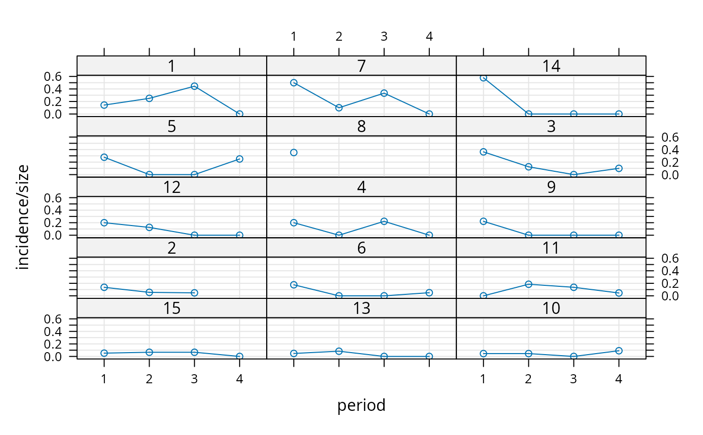
#> glmer> xyplot(incidence/size ~ period|herd, cbpp, type=c('g','p','l'),
#> glmer+ layout=c(3,5), index.cond = function(x,y)max(y))
 #>
#> glmer> (gm1 <- glmer(cbind(incidence, size - incidence) ~ period + (1 | herd),
#> glmer+ data = cbpp, family = binomial))
#> Generalized linear mixed model fit by maximum likelihood (Laplace
#> Approximation) [glmerMod]
#> Family: binomial ( logit )
#> Formula: cbind(incidence, size - incidence) ~ period + (1 | herd)
#> Data: cbpp
#> AIC BIC logLik -2*log(L) df.resid
#> 194.0531 204.1799 -92.0266 184.0531 51
#> Random effects:
#> Groups Name Std.Dev.
#> herd (Intercept) 0.6421
#> Number of obs: 56, groups: herd, 15
#> Fixed Effects:
#> (Intercept) period2 period3 period4
#> -1.3983 -0.9919 -1.1282 -1.5797
#>
#> glmer> ## using nAGQ=0 only gets close to the optimum
#> glmer> (gm1a <- glmer(cbind(incidence, size - incidence) ~ period + (1 | herd),
#> glmer+ cbpp, binomial, nAGQ = 0))
#> Generalized linear mixed model fit by maximum likelihood (Adaptive
#> Gauss-Hermite Quadrature, nAGQ = 0) [glmerMod]
#> Family: binomial ( logit )
#> Formula: cbind(incidence, size - incidence) ~ period + (1 | herd)
#> Data: cbpp
#> AIC BIC logLik -2*log(L) df.resid
#> 194.1087 204.2355 -92.0543 184.1087 51
#> Random effects:
#> Groups Name Std.Dev.
#> herd (Intercept) 0.6418
#> Number of obs: 56, groups: herd, 15
#> Fixed Effects:
#> (Intercept) period2 period3 period4
#> -1.3605 -0.9762 -1.1111 -1.5597
#>
#> glmer> ## using nAGQ = 9 provides a better evaluation of the deviance
#> glmer> ## Currently the internal calculations use the sum of deviance residuals,
#> glmer> ## which is not directly comparable with the nAGQ=0 or nAGQ=1 result.
#> glmer> ## 'verbose = 1' monitors iteratin a bit; (verbose = 2 does more):
#> glmer> (gm1a <- glmer(cbind(incidence, size - incidence) ~ period + (1 | herd),
#> glmer+ cbpp, binomial, verbose = 1, nAGQ = 9))
#> start par. = 1 fn = 186.7231
#> At return
#> eval: 18 fn: 184.10869 par: 0.641839
#> (NM) 20: f = 100.035 at 0.65834 -1.40366 -0.973379 -1.12553 -1.51926
#> (NM) 40: f = 100.012 at 0.650182 -1.39827 -0.993156 -1.11768 -1.57305
#> (NM) 60: f = 100.011 at 0.649102 -1.39735 -0.999034 -1.13415 -1.57634
#> (NM) 80: f = 100.01 at 0.647402 -1.39987 -0.987353 -1.12767 -1.57516
#> (NM) 100: f = 100.01 at 0.64823 -1.4 -0.991134 -1.12755 -1.58048
#> (NM) 120: f = 100.01 at 0.647543 -1.39916 -0.991869 -1.12839 -1.57993
#> (NM) 140: f = 100.01 at 0.647452 -1.39935 -0.991366 -1.12764 -1.57936
#> (NM) 160: f = 100.01 at 0.647519 -1.39925 -0.991348 -1.12784 -1.57948
#> (NM) 180: f = 100.01 at 0.647513 -1.39924 -0.991381 -1.12783 -1.57947
#> Generalized linear mixed model fit by maximum likelihood (Adaptive
#> Gauss-Hermite Quadrature, nAGQ = 9) [glmerMod]
#> Family: binomial ( logit )
#> Formula: cbind(incidence, size - incidence) ~ period + (1 | herd)
#> Data: cbpp
#> AIC BIC logLik -2*log(L) df.resid
#> 110.0100 120.1368 -50.0050 100.0100 51
#> Random effects:
#> Groups Name Std.Dev.
#> herd (Intercept) 0.6475
#> Number of obs: 56, groups: herd, 15
#> Fixed Effects:
#> (Intercept) period2 period3 period4
#> -1.3992 -0.9914 -1.1278 -1.5795
#>
#> glmer> ## GLMM with individual-level variability (accounting for overdispersion)
#> glmer> ## For this data set the model is the same as one allowing for a period:herd
#> glmer> ## interaction, which the plot indicates could be needed.
#> glmer> cbpp$obs <- 1:nrow(cbpp)
#>
#> glmer> (gm2 <- glmer(cbind(incidence, size - incidence) ~ period +
#> glmer+ (1 | herd) + (1|obs),
#> glmer+ family = binomial, data = cbpp))
#> Generalized linear mixed model fit by maximum likelihood (Laplace
#> Approximation) [glmerMod]
#> Family: binomial ( logit )
#> Formula: cbind(incidence, size - incidence) ~ period + (1 | herd) + (1 |
#> obs)
#> Data: cbpp
#> AIC BIC logLik -2*log(L) df.resid
#> 186.6383 198.7904 -87.3192 174.6383 50
#> Random effects:
#> Groups Name Std.Dev.
#> obs (Intercept) 0.8911
#> herd (Intercept) 0.1840
#> Number of obs: 56, groups: obs, 56; herd, 15
#> Fixed Effects:
#> (Intercept) period2 period3 period4
#> -1.500 -1.226 -1.329 -1.866
#>
#> glmer> anova(gm1,gm2)
#> Data: cbpp
#> Models:
#> gm1: cbind(incidence, size - incidence) ~ period + (1 | herd)
#> gm2: cbind(incidence, size - incidence) ~ period + (1 | herd) + (1 | obs)
#> npar AIC BIC logLik -2*log(L) Chisq Df Pr(>Chisq)
#> gm1 5 194.05 204.18 -92.027 184.05
#> gm2 6 186.64 198.79 -87.319 174.64 9.4148 1 0.002152 **
#> ---
#> Signif. codes: 0 ‘***’ 0.001 ‘**’ 0.01 ‘*’ 0.05 ‘.’ 0.1 ‘ ’ 1
#>
#> glmer> ## glmer and glm log-likelihoods are consistent
#> glmer> gm1Devfun <- update(gm1,devFunOnly=TRUE)
#>
#> glmer> gm0 <- glm(cbind(incidence, size - incidence) ~ period,
#> glmer+ family = binomial, data = cbpp)
#>
#> glmer> ## evaluate GLMM deviance at RE variance=theta=0, beta=(GLM coeffs)
#> glmer> gm1Dev0 <- gm1Devfun(c(0,coef(gm0)))
#>
#> glmer> ## compare
#> glmer> stopifnot(all.equal(gm1Dev0,c(-2*logLik(gm0))))
#>
#> glmer> ## the toenail oncholysis data from Backer et al 1998
#> glmer> ## these data are notoriously difficult to fit
#> glmer> ## Not run:
#> glmer> ##D if (require("HSAUR3")) {
#> glmer> ##D gm2 <- glmer(outcome~treatment*visit+(1|patientID),
#> glmer> ##D data=toenail,
#> glmer> ##D family=binomial,nAGQ=20)
#> glmer> ##D }
#> glmer> ## End(Not run)
#> glmer>
#> glmer>
#> glmer>
linearHypothesis(gm1, matchCoefs(gm1, "period"))
#>
#> Linear hypothesis test:
#> period2 = 0
#> period3 = 0
#> period4 = 0
#>
#> Model 1: restricted model
#> Model 2: cbind(incidence, size - incidence) ~ period + (1 | herd)
#>
#> Df Chisq Pr(>Chisq)
#> 1
#> 2 3 25.488 1.221e-05 ***
#> ---
#> Signif. codes: 0 ‘***’ 0.001 ‘**’ 0.01 ‘*’ 0.05 ‘.’ 0.1 ‘ ’ 1
# \dontrun{}
if (require(nnet)){
print(m <- multinom(partic ~ hincome + children, data=Womenlf))
print(coefs <- as.vector(outer(c("not.work.", "parttime."),
c("hincome", "childrenpresent"),
paste0)))
linearHypothesis(m, coefs) # ominbus Wald test
}
#> Loading required package: nnet
#> # weights: 12 (6 variable)
#> initial value 288.935032
#> iter 10 value 211.441198
#> final value 211.440963
#> converged
#> Call:
#> multinom(formula = partic ~ hincome + children, data = Womenlf)
#>
#> Coefficients:
#> (Intercept) hincome childrenpresent
#> not.work -1.982826 0.09723134 2.558598
#> parttime -3.415105 0.10411973 2.580127
#>
#> Residual Deviance: 422.8819
#> AIC: 434.8819
#> [1] "not.work.hincome" "parttime.hincome"
#> [3] "not.work.childrenpresent" "parttime.childrenpresent"
#>
#> Linear hypothesis test:
#> not.work.hincome = 0
#> parttime.hincome = 0
#> not.work.childrenpresent = 0
#> parttime.childrenpresent = 0
#>
#> Model 1: restricted model
#> Model 2: partic ~ hincome + children
#>
#> Df Chisq Pr(>Chisq)
#> 1
#> 2 4 58.435 6.183e-12 ***
#> ---
#> Signif. codes: 0 ‘***’ 0.001 ‘**’ 0.01 ‘*’ 0.05 ‘.’ 0.1 ‘ ’ 1
#>
#> glmer> (gm1 <- glmer(cbind(incidence, size - incidence) ~ period + (1 | herd),
#> glmer+ data = cbpp, family = binomial))
#> Generalized linear mixed model fit by maximum likelihood (Laplace
#> Approximation) [glmerMod]
#> Family: binomial ( logit )
#> Formula: cbind(incidence, size - incidence) ~ period + (1 | herd)
#> Data: cbpp
#> AIC BIC logLik -2*log(L) df.resid
#> 194.0531 204.1799 -92.0266 184.0531 51
#> Random effects:
#> Groups Name Std.Dev.
#> herd (Intercept) 0.6421
#> Number of obs: 56, groups: herd, 15
#> Fixed Effects:
#> (Intercept) period2 period3 period4
#> -1.3983 -0.9919 -1.1282 -1.5797
#>
#> glmer> ## using nAGQ=0 only gets close to the optimum
#> glmer> (gm1a <- glmer(cbind(incidence, size - incidence) ~ period + (1 | herd),
#> glmer+ cbpp, binomial, nAGQ = 0))
#> Generalized linear mixed model fit by maximum likelihood (Adaptive
#> Gauss-Hermite Quadrature, nAGQ = 0) [glmerMod]
#> Family: binomial ( logit )
#> Formula: cbind(incidence, size - incidence) ~ period + (1 | herd)
#> Data: cbpp
#> AIC BIC logLik -2*log(L) df.resid
#> 194.1087 204.2355 -92.0543 184.1087 51
#> Random effects:
#> Groups Name Std.Dev.
#> herd (Intercept) 0.6418
#> Number of obs: 56, groups: herd, 15
#> Fixed Effects:
#> (Intercept) period2 period3 period4
#> -1.3605 -0.9762 -1.1111 -1.5597
#>
#> glmer> ## using nAGQ = 9 provides a better evaluation of the deviance
#> glmer> ## Currently the internal calculations use the sum of deviance residuals,
#> glmer> ## which is not directly comparable with the nAGQ=0 or nAGQ=1 result.
#> glmer> ## 'verbose = 1' monitors iteratin a bit; (verbose = 2 does more):
#> glmer> (gm1a <- glmer(cbind(incidence, size - incidence) ~ period + (1 | herd),
#> glmer+ cbpp, binomial, verbose = 1, nAGQ = 9))
#> start par. = 1 fn = 186.7231
#> At return
#> eval: 18 fn: 184.10869 par: 0.641839
#> (NM) 20: f = 100.035 at 0.65834 -1.40366 -0.973379 -1.12553 -1.51926
#> (NM) 40: f = 100.012 at 0.650182 -1.39827 -0.993156 -1.11768 -1.57305
#> (NM) 60: f = 100.011 at 0.649102 -1.39735 -0.999034 -1.13415 -1.57634
#> (NM) 80: f = 100.01 at 0.647402 -1.39987 -0.987353 -1.12767 -1.57516
#> (NM) 100: f = 100.01 at 0.64823 -1.4 -0.991134 -1.12755 -1.58048
#> (NM) 120: f = 100.01 at 0.647543 -1.39916 -0.991869 -1.12839 -1.57993
#> (NM) 140: f = 100.01 at 0.647452 -1.39935 -0.991366 -1.12764 -1.57936
#> (NM) 160: f = 100.01 at 0.647519 -1.39925 -0.991348 -1.12784 -1.57948
#> (NM) 180: f = 100.01 at 0.647513 -1.39924 -0.991381 -1.12783 -1.57947
#> Generalized linear mixed model fit by maximum likelihood (Adaptive
#> Gauss-Hermite Quadrature, nAGQ = 9) [glmerMod]
#> Family: binomial ( logit )
#> Formula: cbind(incidence, size - incidence) ~ period + (1 | herd)
#> Data: cbpp
#> AIC BIC logLik -2*log(L) df.resid
#> 110.0100 120.1368 -50.0050 100.0100 51
#> Random effects:
#> Groups Name Std.Dev.
#> herd (Intercept) 0.6475
#> Number of obs: 56, groups: herd, 15
#> Fixed Effects:
#> (Intercept) period2 period3 period4
#> -1.3992 -0.9914 -1.1278 -1.5795
#>
#> glmer> ## GLMM with individual-level variability (accounting for overdispersion)
#> glmer> ## For this data set the model is the same as one allowing for a period:herd
#> glmer> ## interaction, which the plot indicates could be needed.
#> glmer> cbpp$obs <- 1:nrow(cbpp)
#>
#> glmer> (gm2 <- glmer(cbind(incidence, size - incidence) ~ period +
#> glmer+ (1 | herd) + (1|obs),
#> glmer+ family = binomial, data = cbpp))
#> Generalized linear mixed model fit by maximum likelihood (Laplace
#> Approximation) [glmerMod]
#> Family: binomial ( logit )
#> Formula: cbind(incidence, size - incidence) ~ period + (1 | herd) + (1 |
#> obs)
#> Data: cbpp
#> AIC BIC logLik -2*log(L) df.resid
#> 186.6383 198.7904 -87.3192 174.6383 50
#> Random effects:
#> Groups Name Std.Dev.
#> obs (Intercept) 0.8911
#> herd (Intercept) 0.1840
#> Number of obs: 56, groups: obs, 56; herd, 15
#> Fixed Effects:
#> (Intercept) period2 period3 period4
#> -1.500 -1.226 -1.329 -1.866
#>
#> glmer> anova(gm1,gm2)
#> Data: cbpp
#> Models:
#> gm1: cbind(incidence, size - incidence) ~ period + (1 | herd)
#> gm2: cbind(incidence, size - incidence) ~ period + (1 | herd) + (1 | obs)
#> npar AIC BIC logLik -2*log(L) Chisq Df Pr(>Chisq)
#> gm1 5 194.05 204.18 -92.027 184.05
#> gm2 6 186.64 198.79 -87.319 174.64 9.4148 1 0.002152 **
#> ---
#> Signif. codes: 0 ‘***’ 0.001 ‘**’ 0.01 ‘*’ 0.05 ‘.’ 0.1 ‘ ’ 1
#>
#> glmer> ## glmer and glm log-likelihoods are consistent
#> glmer> gm1Devfun <- update(gm1,devFunOnly=TRUE)
#>
#> glmer> gm0 <- glm(cbind(incidence, size - incidence) ~ period,
#> glmer+ family = binomial, data = cbpp)
#>
#> glmer> ## evaluate GLMM deviance at RE variance=theta=0, beta=(GLM coeffs)
#> glmer> gm1Dev0 <- gm1Devfun(c(0,coef(gm0)))
#>
#> glmer> ## compare
#> glmer> stopifnot(all.equal(gm1Dev0,c(-2*logLik(gm0))))
#>
#> glmer> ## the toenail oncholysis data from Backer et al 1998
#> glmer> ## these data are notoriously difficult to fit
#> glmer> ## Not run:
#> glmer> ##D if (require("HSAUR3")) {
#> glmer> ##D gm2 <- glmer(outcome~treatment*visit+(1|patientID),
#> glmer> ##D data=toenail,
#> glmer> ##D family=binomial,nAGQ=20)
#> glmer> ##D }
#> glmer> ## End(Not run)
#> glmer>
#> glmer>
#> glmer>
linearHypothesis(gm1, matchCoefs(gm1, "period"))
#>
#> Linear hypothesis test:
#> period2 = 0
#> period3 = 0
#> period4 = 0
#>
#> Model 1: restricted model
#> Model 2: cbind(incidence, size - incidence) ~ period + (1 | herd)
#>
#> Df Chisq Pr(>Chisq)
#> 1
#> 2 3 25.488 1.221e-05 ***
#> ---
#> Signif. codes: 0 ‘***’ 0.001 ‘**’ 0.01 ‘*’ 0.05 ‘.’ 0.1 ‘ ’ 1
# \dontrun{}
if (require(nnet)){
print(m <- multinom(partic ~ hincome + children, data=Womenlf))
print(coefs <- as.vector(outer(c("not.work.", "parttime."),
c("hincome", "childrenpresent"),
paste0)))
linearHypothesis(m, coefs) # ominbus Wald test
}
#> Loading required package: nnet
#> # weights: 12 (6 variable)
#> initial value 288.935032
#> iter 10 value 211.441198
#> final value 211.440963
#> converged
#> Call:
#> multinom(formula = partic ~ hincome + children, data = Womenlf)
#>
#> Coefficients:
#> (Intercept) hincome childrenpresent
#> not.work -1.982826 0.09723134 2.558598
#> parttime -3.415105 0.10411973 2.580127
#>
#> Residual Deviance: 422.8819
#> AIC: 434.8819
#> [1] "not.work.hincome" "parttime.hincome"
#> [3] "not.work.childrenpresent" "parttime.childrenpresent"
#>
#> Linear hypothesis test:
#> not.work.hincome = 0
#> parttime.hincome = 0
#> not.work.childrenpresent = 0
#> parttime.childrenpresent = 0
#>
#> Model 1: restricted model
#> Model 2: partic ~ hincome + children
#>
#> Df Chisq Pr(>Chisq)
#> 1
#> 2 4 58.435 6.183e-12 ***
#> ---
#> Signif. codes: 0 ‘***’ 0.001 ‘**’ 0.01 ‘*’ 0.05 ‘.’ 0.1 ‘ ’ 1