Methods Functions to Support boot Objects

The Boot function in the car package uses the boot function from the boot package to do a straightforward case or residual bootstrap for many regression objects. These are method functions for standard generics to summarize the results of the bootstrap. Other tools for this purpose are available in the boot package.

Usage

# S3 method for class 'boot'
hist(x, parm, layout = NULL, ask, main = "", freq = FALSE,
    estPoint = TRUE, point.col = carPalette()[1], point.lty = 2, point.lwd = 2,
    estDensity = !freq, den.col = carPalette()[2], den.lty = 1, den.lwd = 2,
    estNormal = !freq, nor.col = carPalette()[3], nor.lty = 2, nor.lwd = 2,
    ci = c("bca", "none", "perc", "norm"), level = 0.95, 
    legend = c("top", "none", "separate"), box = TRUE, ...)

# S3 method for class 'boot'
summary(object, parm, high.moments = FALSE, extremes = FALSE, ...)

# S3 method for class 'boot'
confint(object, parm, level = 0.95, type = c("bca", "norm",
    "basic", "perc"), ...)

# S3 method for class 'boot'
Confint(object, parm, level = 0.95, type = c("bca", "norm",
    "basic", "perc"), ...)

# S3 method for class 'boot'
vcov(object, use="complete.obs", ...)

Arguments

x, object: An object created by a call to boot in the boot package, or to Boot in the car package of class "boot".
parm: A vector of numbers or coefficient names giving the coefficients for which a histogram or confidence interval is desired. If numbers are used, 1 corresponds to the intercept, if any. The default is all coefficients.
layout: If set to a value like c(1, 1) or c(4, 3), the layout of the graph will have this many rows and columns. If not set, the program will select an appropriate layout. If the number of graphs exceed nine, you must select the layout yourself, or you will get a maximum of nine per page. If layout=NA, the function does not set the layout and the user can use the par function to control the layout, for example to have plots from two models in the same graphics window.
ask: If TRUE, ask the user before drawing the next plot; if FALSE, don't ask.
main: Main title for the graphs. The default is main="" for no title.
freq: The default for the generic hist function is freq=TRUE to give a frequency histogram. The default for hist.boot is freq=FALSE to give a density histogram. A density estimate and/or a fitted normal density can be added to the graph if freq=FALSE but not if freq=TRUE.
estPoint, point.col, point.lty, point.lwd: If estPoint=TRUE, the default, a vertical line is drawn on the histgram at the value of the point estimate computed from the complete data. The remaining three optional arguments set the color, line type and line width of the line that is drawn.
estDensity, den.col, den.lty, den.lwd: If estDensity=TRUE andfreq=FALSE, the default, a kernel density estimate is drawn on the plot with a call to the density function with no additional arguments. The remaining three optional arguments set the color, line type and line width of the lines that are drawn.
estNormal, nor.col, nor.lty, nor.lwd: If estNormal=TRUE andfreq=FALSE, the default, a normal density with mean and sd computed from the data is drawn on the plot. The remaining three optional arguments set the color, line type and line width of the lines that are drawn.
ci: A confidence interval based on the bootstrap will be added to the histogram using the BCa method if ci="bca" the percentile method if ci="perc", or the normal method if ci="norm". No interval is drawn if ci="none". The default is "bca". The interval is indicated by a thick horizontal line at y=0. For some bootstraps the BCa method is unavailable, in which case a warning is issued and ci="perc" is substituted. If you wish to see all the options at once, see boot.ci. The normal method is computed as the (estimate from the original data) minus the bootstrap bias plus or minus the standard deviation of the bootstrap replicates times the appropriate quantile of the standard normal distribution.
legend: A legend can be added to the (array of) histograms. The value “top” puts at the top-left of the plots. The value “separate” puts the legend in its own graph following all the histograms. The value “none” suppresses the legend.
box: Add a box around each histogram.
...: Additional arguments passed to hist; for other methods this is included for compatibility with the generic method. For example, the argument border=par()$bg in hist will draw the histogram transparently, leaving only the density estimates. With the vcov function, the additional arguments are passed to cov. See the Value section, below.
high.moments: Should the skewness and kurtosis be included in the summary? Default is FALSE.
extremes: Should the minimum, maximum and range be included in the summary? Default is FALSE.
level: Confidence level, a number between 0 and 1. In confint, level can be a vector; for example level=c(.50, .90, .95) will return the following estimated quantiles: c(.025, .05, .25, .75, .95, .975).
type: Selects the confidence interval type. The types implemented are the "percentile" method, which uses the function quantile to return the appropriate quantiles for the confidence limit specified, the default bca which uses the bias-corrected and accelerated method presented by Efron and Tibshirani (1993, Chapter 14). For the other types, see the documentation for boot.
use: The default use="complete.obs" for vcov computes a bootstrap covariance matrix by deleting bootstraps that returned NAs. Setting use to anything else will result in a matrix of NAs.

Value

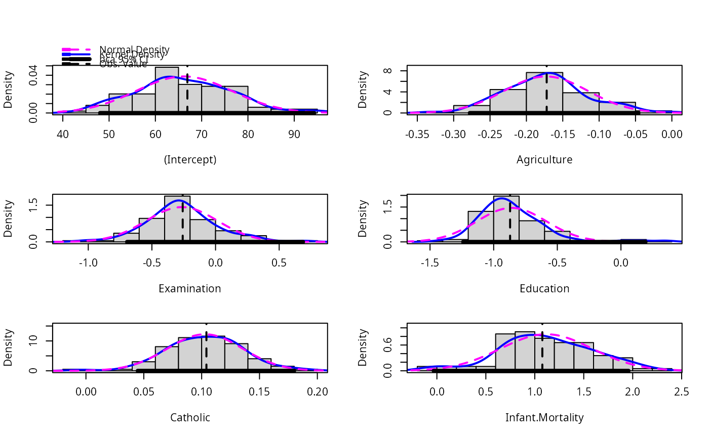
hist is used for the side-effect of drawing an array of historgams of each column of the first argument. summary returns a matrix of summary statistics for each of the columns in the bootstrap object. The confint method returns confidence intervals. Confint appends the estimates based on the original fitted model to the left of the confidence intervals.

The function vcov returns the sample covariance of the bootstrap sample estimates, by default skipping any bootstrap samples that returned NA.

References

Efron, B. and Tibsharini, R. (1993) An Introduction to the Bootstrap. New York: Chapman and Hall.

Fox, J. and Weisberg, S. (2019) An R Companion to Applied Regression, Third Edition. Thousand Oaks: Sage.

Fox, J. and Weisberg, S. (2018) Bootstrapping Regression Models in R, https://www.john-fox.ca/Companion/appendices/Appendix-Bootstrapping.pdf.

Weisberg, S. (2013) Applied Linear Regression, Fourth Edition, Wiley

Author

Sanford Weisberg, sandy@umn.edu

Examples

m1 <- lm(Fertility ~ ., swiss)
betahat.boot <- Boot(m1, R=99) # 99 bootstrap samples--too small to be useful
summary(betahat.boot)  # default summary
#> 
#> Number of bootstrap replications R = 99 
#>                  original    bootBias    bootSE  bootMed
#> (Intercept)      66.91518 -0.72987798 10.298911 65.11385
#> Agriculture      -0.17211 -0.00094133  0.057571 -0.17374
#> Examination      -0.25801 -0.00651854  0.281014 -0.27966
#> Education        -0.87094  0.01214621  0.272658 -0.90280
#> Catholic          0.10412 -0.00119656  0.032615  0.10294
#> Infant.Mortality  1.07705  0.04131993  0.469178  1.09702
confint(betahat.boot)
#> Warning: extreme order statistics used as endpoints
#> Bootstrap bca confidence intervals
#> 
#>                        2.5 %      97.5 %
#> (Intercept)      48.04489391 94.32573968
#> Agriculture      -0.27785428 -0.04581786
#> Examination      -0.69551062  0.68781876
#> Education        -1.24023899  0.19361408
#> Catholic          0.04470735  0.17997837
#> Infant.Mortality -0.03324832  1.95792293
hist(betahat.boot)
#> Warning: extreme order statistics used as endpoints

Methods Functions to Support `boot` Objects