Graph the profile log-likelihood for Box-Cox transformations in 1D, or in 2D with the bcnPower family.

Computes and optionally plots profile log-likelihoods for the parameter of the Box-Cox power family, the Yeo-Johnson power family, or for either of the parameters in a bcnPower family. This is a slight generalization of the boxcox function in the MASS package that allows for families of transformations other than the Box-Cox power family. the boxCox2d function produces a contour plot of the two-dimensional likelihood profile for the bcnPower family.

Usage

boxCox(object, ...)

# Default S3 method
boxCox(object,
        lambda = seq(-2, 2, 1/10), plotit = TRUE,
        interp = plotit, eps = 1/50,
        xlab=NULL, ylab=NULL, main= "Profile Log-likelihood",
        family="bcPower",
        param=c("lambda", "gamma"), gamma=NULL,
        grid=TRUE, ...)

# S3 method for class 'formula'
boxCox(object, lambda = seq(-2, 2, 1/10), plotit = TRUE, family = "bcPower",
    param = c("lambda", "gamma"), gamma = NULL, grid = TRUE,
    ...)

# S3 method for class 'lm'
boxCox(object, lambda = seq(-2, 2, 1/10), plotit = TRUE, ...)

boxCox2d(x, ksds = 4, levels = c(0.5, 0.95, 0.99, 0.999),
                 main = "bcnPower Log-likelihood", grid=TRUE, ...)

Arguments

object: a formula or fitted model object of class lm or aov.
lambda: vector of values of \(\lambda\), with default (-2, 2) in steps of 0.1, where the profile log-likelihood will be evaluated.
plotit: logical which controls whether the result should be plotted; default TRUE.
interp: logical which controls whether spline interpolation is used. Default to TRUE if plotting with lambda of length less than 100.
eps: Tolerance for lambda = 0; defaults to 0.02.
xlab: defaults to "lambda" or "gamma".
ylab: defaults to "log-Likelihood" or for bcnPower family to the appropriate label.
family: Defaults to "bcPower" for the Box-Cox power family of transformations. If set to "yjPower" the Yeo-Johnson family, which permits negative responses, is used. If set to bcnPower the function gives the profile log-likelihood for the parameter selected via param.
param: Relevant only to family="bcnPower", produces a profile log-likelihood for the parameter selected, maximizing over the remaining parameter.
gamma: For use when the family="bcnPower", param="gamma". If this is a vector of positive values, then the profile log-likelihood for the location (or start) parameter in the bcnPower family is evaluated at these values of gamma. If gamma is NULL, then evaulation is done at 100 equally spaced points between min(.01, gmax - 3*sd) and gmax + 3*sd, where gmax is the maximimum likelihood estimate of gamma, and sd is the sd of the response. See bcnPower for the definition of gamma.
grid: If TRUE, the default, a light-gray background grid is put on the graph.
...: additional arguments passed to plot, or to contour with boxCox2d.
x: An object created by a call to powerTransform using family="bcnPower".
ksds: Contour plotting of the log-likelihood surface will cover plus of minus ksds standard deviations on each axis.
levels: Contours will be drawn at the values of levels. For example, levels=c(.5, .99) would display two contours, at the 50% level and at the 99% level.
main: Title for the contour plot or the profile log-likelihood plot

Details

The boxCox function is an elaboration of the boxcox function in the MASS package. The first 7 arguments are the same as in boxcox, and if the argument family="bcPower" is used, the result is essentially identical to the function in MASS. Two additional families are the yjPower and bcnPower families that allow a few values of the response to be non-positive. The bcnPower family has two parameters: a power \(\lambda\) and a start or location parameter \(\gamma\), and the boxCox function can be used to obtain a profile log-likelihood for either parameter with \(\lambda\) as the default. Alternatively, the boxCox2d function can be used to get a contour plot of the profile log-likelihood.

Value

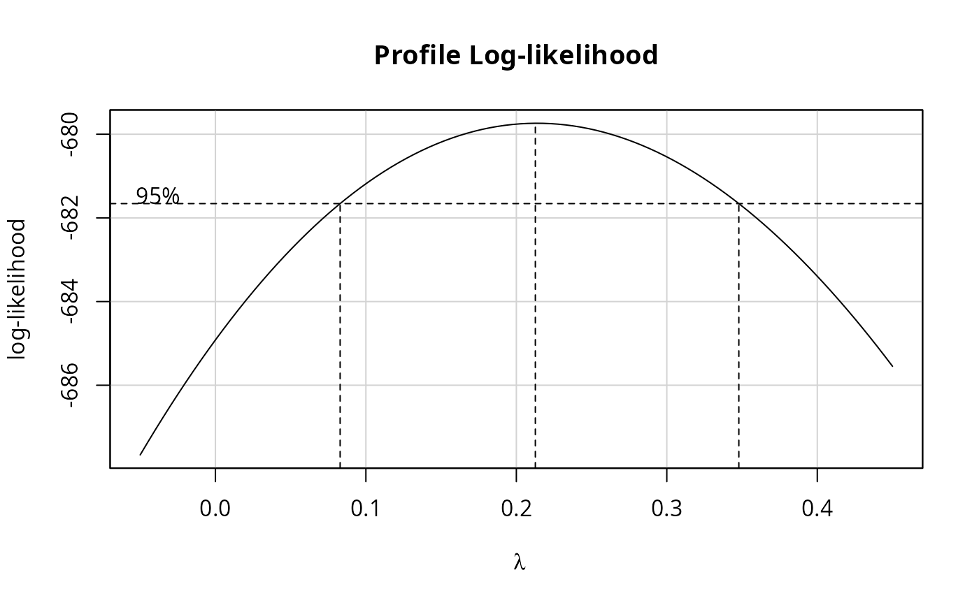
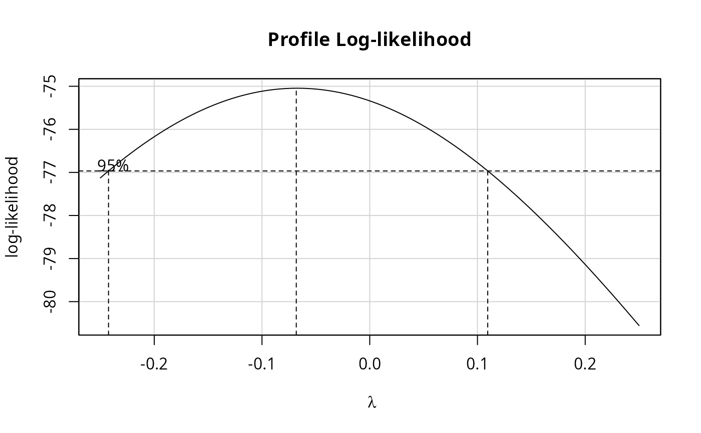
Both functions ae designed for their side effects of drawing a graph. The boxCox function returns a list of the lambda (or possibly, gamma) vector and the computed profile log-likelihood vector, invisibly if the result is plotted. If plotit=TRUE plots log-likelihood vs lambda and indicates a 95% confidence interval about the maximum observed value of lambda. If interp=TRUE, spline interpolation is used to give a smoother plot.

References

Box, G. E. P. and Cox, D. R. (1964) An analysis of transformations. Journal of the Royal Statisistical Society, Series B. 26 211-46.

Cook, R. D. and Weisberg, S. (1999) Applied Regression Including Computing and Graphics. Wiley.

Fox, J. (2016) Applied Regression Analysis and Generalized Linear Models, Third Edition. Sage.

Fox, J. and Weisberg, S. (2019) An R Companion to Applied Regression, Third Edition, Sage.

Hawkins, D. and Weisberg, S. (2017) Combining the Box-Cox Power and Generalized Log Transformations to Accomodate Nonpositive Responses In Linear and Mixed-Effects Linear Models South African Statistics Journal, 51, 317-328.

Weisberg, S. (2014) Applied Linear Regression, Fourth Edition, Wiley.

Yeo, I. and Johnson, R. (2000) A new family of power transformations to improve normality or symmetry. Biometrika, 87, 954-959.

Author

Sanford Weisberg, <sandy@umn.edu>

Examples

  with(trees, boxCox(Volume ~ log(Height) + log(Girth), data = trees,
         lambda = seq(-0.25, 0.25, length = 10)))
#> Warning: "data" is not a graphical parameter
#> Warning: "data" is not a graphical parameter
#> Warning: "data" is not a graphical parameter
#> Warning: "data" is not a graphical parameter
#> Warning: "data" is not a graphical parameter
#> Warning: "data" is not a graphical parameter


  data("quine", package = "MASS")
  with(quine, boxCox(Days ~ Eth*Sex*Age*Lrn, 
         lambda = seq(-0.05, 0.45, len = 20), family="yjPower"))