Binomial confidence intervals using Bayesian inference

Uses a beta prior on the probability of success for a binomial distribution, determines a two-sided confidence interval from a beta posterior. A plotting function is also provided to show the probability regions defined by each confidence interval.

binom.bayes(x, n,
            conf.level = 0.95,
            type = c("highest", "central"),
            prior.shape1 = 0.5,
            prior.shape2 = 0.5,
            tol = .Machine$double.eps^0.5,
            maxit = 1000, ...)

binom.bayes.densityplot(bayes,
                        npoints = 500,
                        fill.central = "lightgray",
                        fill.lower = "steelblue",
                        fill.upper = fill.lower,
                        alpha = 0.8, ...)

Arguments

x: Vector of number of successes in the binomial experiment.
n: Vector of number of independent trials in the binomial experiment.
conf.level: The level of confidence to be used in the confidence interval.
type: The type of confidence interval (see Details).
prior.shape1: The value of the first shape parameter to be used in the prior beta.
prior.shape2: The value of the second shape parameter to be used in the prior beta.
tol: A tolerance to be used in determining the highest probability density interval.
maxit: Maximum number of iterations to be used in determining the highest probability interval.
bayes: The output data.frame from binom.bayes.
npoints: The number of points to use to draw the density curves. Higher numbers give smoother densities.
fill.central: The color for the central density.
fill.lower,fill.upper: The color(s) for the upper and lower density.
alpha: The alpha value for controlling transparency.
...: Ignored.

Details

Using the conjugate beta prior on the distribution of p (the probability of success) in a binomial experiment, constructs a confidence interval from the beta posterior. From Bayes theorem the posterior distribution of p given the data x is:

p|x ~ Beta(x + prior.shape1, n - x + prior.shape2)

The default prior is Jeffrey's prior which is a Beta(0.5, 0.5) distribution. Thus the posterior mean is (x + 0.5)/(n + 1).

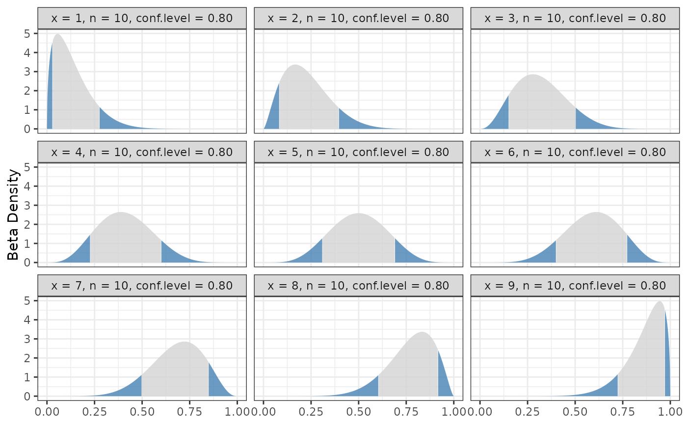
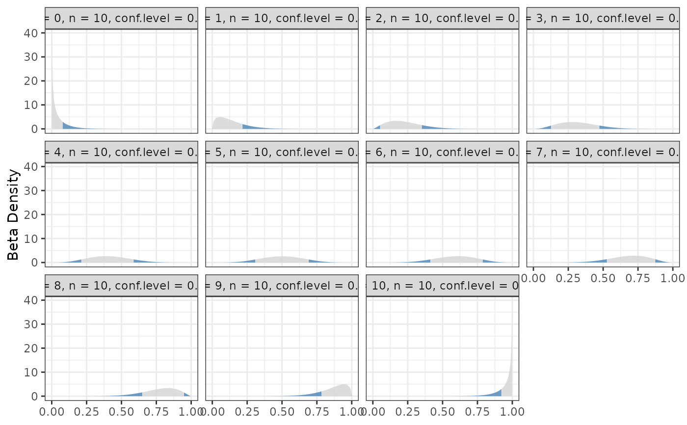
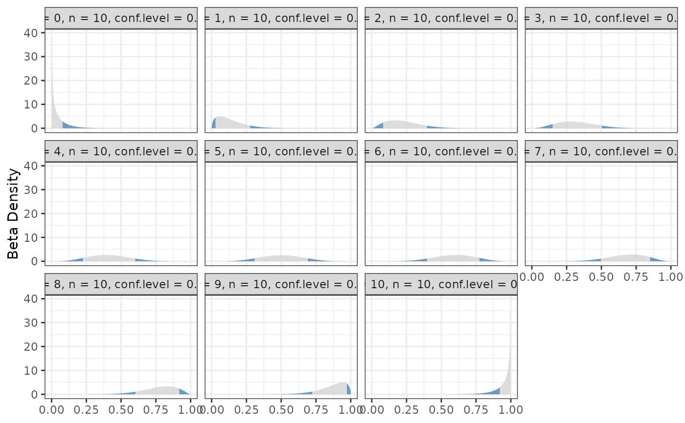
The default type of interval constructed is "highest" which computes the highest probability density (hpd) interval which assures the shortest interval possible. The hpd intervals will achieve a probability that is within tol of the specified conf.level. Setting type to "central" constructs intervals that have equal tail probabilities.

If 0 or n successes are observed, a one-sided confidence interval is returned.

Value

For binom.bayes, a data.frame containing the observed proportions and the lower and upper bounds of the confidence interval.

For binom.bayes.densityplot, a ggplot object that can printed to a graphics device, or have additional layers added.

References

Gelman, A., Carlin, J. B., Stern, H. S., and Rubin, D. B. (1997) Bayesian Data Analysis, London, U.K.: Chapman and Hall.

Author

Sundar Dorai-Raj (sdorairaj@gmail.com)

Examples

# Example using highest probability density.
hpd <- binom.bayes(
  x = 0:10, n = 10, type = "highest", conf.level = 0.8, tol = 1e-9)
print(hpd)
#>    method  x  n shape1 shape2       mean       lower     upper sig
#> 1   bayes  0 10    0.5   10.5 0.04545455 0.000000000 0.0769566 0.2
#> 2   bayes  1 10    1.5    9.5 0.13636364 0.003771457 0.2145408 0.2
#> 3   bayes  2 10    2.5    8.5 0.22727273 0.053633312 0.3494770 0.2
#> 4   bayes  3 10    3.5    7.5 0.31818182 0.127646004 0.4728042 0.2
#> 5   bayes  4 10    4.5    6.5 0.40909091 0.214091147 0.5858428 0.2
#> 6   bayes  5 10    5.5    5.5 0.50000000 0.309892028 0.6901080 0.2
#> 7   bayes  6 10    6.5    4.5 0.59090909 0.414157185 0.7859089 0.2
#> 8   bayes  7 10    7.5    3.5 0.68181818 0.527195809 0.8723540 0.2
#> 9   bayes  8 10    8.5    2.5 0.77272727 0.650522982 0.9463667 0.2
#> 10  bayes  9 10    9.5    1.5 0.86363636 0.785459228 0.9962285 0.2
#> 11  bayes 10 10   10.5    0.5 0.95454545 0.923043403 1.0000000 0.2
binom.bayes.densityplot(hpd)
#> Loading required namespace: ggplot2
#> Warning: `aes_string()` was deprecated in ggplot2 3.0.0.
#> ℹ Please use tidy evaluation idioms with `aes()`.
#> ℹ See also `vignette("ggplot2-in-packages")` for more information.
#> ℹ The deprecated feature was likely used in the binom package.
#>   Please report the issue to the authors.

# Remove the extremes from the plot since they make things hard
# to see.
binom.bayes.densityplot(hpd[hpd$x != 0 & hpd$x != 10, ])


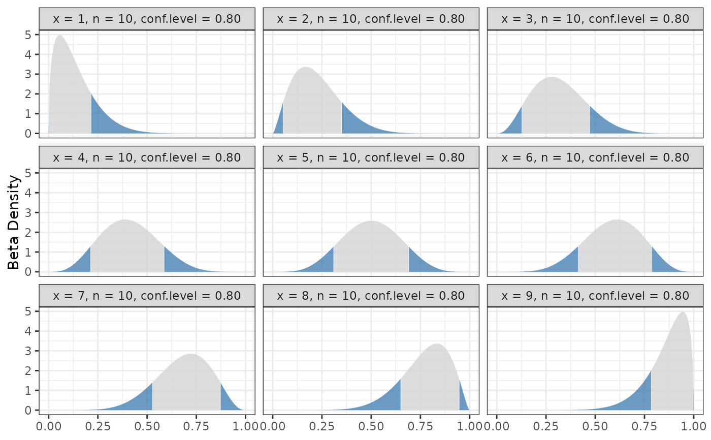# Example using central probability.
central <- binom.bayes(
  x = 0:10, n = 10, type = "central", conf.level = 0.8, tol = 1e-9)
print(central)
#>    method  x  n shape1 shape2       mean      lower     upper sig
#> 1   bayes  0 10    0.5   10.5 0.04545455 0.00000000 0.0769566 0.2
#> 2   bayes  1 10    1.5    9.5 0.13636364 0.02954113 0.2745618 0.2
#> 3   bayes  2 10    2.5    8.5 0.22727273 0.08361516 0.3948296 0.2
#> 4   bayes  3 10    3.5    7.5 0.31818182 0.15059123 0.5017811 0.2
#> 5   bayes  4 10    4.5    6.5 0.40909091 0.22651679 0.5996844 0.2
#> 6   bayes  5 10    5.5    5.5 0.50000000 0.30989203 0.6901080 0.2
#> 7   bayes  6 10    6.5    4.5 0.59090909 0.40031562 0.7734832 0.2
#> 8   bayes  7 10    7.5    3.5 0.68181818 0.49821888 0.8494088 0.2
#> 9   bayes  8 10    8.5    2.5 0.77272727 0.60517036 0.9163848 0.2
#> 10  bayes  9 10    9.5    1.5 0.86363636 0.72543825 0.9704589 0.2
#> 11  bayes 10 10   10.5    0.5 0.95454545 0.92304340 1.0000000 0.2
binom.bayes.densityplot(central)

# Remove the extremes from the plot since they make things hard
# to see.
binom.bayes.densityplot(central[central$x != 0 & central$x != 10, ])