Main Effects Plot for a Row-Column Interaction Model (RCIM)
plotrcim0.RdProduces a main effects plot for Row-Column Interaction Models (RCIMs).
Usage
plotrcim0(object, centered = TRUE, which.plots = c(1, 2),
            hline0 = TRUE, hlty = "dashed", hcol = par()$col, hlwd = par()$lwd,
            rfirst = 1, cfirst = 1,
            rtype = "h", ctype = "h",
            rcex.lab = 1, rcex.axis = 1, rtick = FALSE,
            ccex.lab = 1, ccex.axis = 1, ctick = FALSE,
            rmain = "Row effects", rsub = "",
            rxlab = "", rylab = "Row effects",
            cmain = "Column effects", csub = "",
            cxlab= "", cylab = "Column effects",
            rcol = par()$col, ccol = par()$col,
            no.warning = FALSE, ...)
Arguments
- object
An
rcimobject. This should be of rank-0, i.e., main effects only and no interactions.- which.plots
Numeric, describing which plots are to be plotted. The row effects plot is 1 and the column effects plot is 2. Set the value
0, say, for no plots at all.- centered
Logical. If
TRUEthen the row and column effects are centered (but not scaled) byscale. IfFALSEthen the raw effects are used (of which the first are zero by definition).- hline0, hlty, hcol, hlwd
hline0is logical. IfTRUEthen a horizontal line is plotted at 0 and the other arguments describe this line. Probably havinghline0 = TRUEonly makes sense whencentered = TRUE.- rfirst, cfirst
rfirstis the level of row that is placed first in the row effects plot, etc.- rmain, cmain
Character.
rmainis the main label in the row effects plot, etc.- rtype, ctype, rsub, csub
See the
typeandsubarguments ofplot.default.
- rxlab, rylab, cxlab, cylab
Character. For the row effects plot,
rxlabisxlabandrylabisylab; seepar. Ditto forcxlabandcylabfor the column effects plot.- rcex.lab, ccex.lab
Numeric.
rcex.labiscexfor the row effects plot label, etc.- rcex.axis, ccex.axis
Numeric.
rcex.axisis thecexargument for the row effects axis label, etc.- rtick, ctick
Logical. If
rtick = TRUEthen add ticks to the row effects plot, etc.- rcol, ccol
rcolgive a colour for the row effects plot, etc.- no.warning
Logical. If
TRUEthen no warning is issued if the model is not rank-0.
- ...
Arguments fed into
plot.default, etc.
Details
This function plots the row and column effects of a rank-0 RCIM.
As the result is a main effects plot of a regression analysis, its
interpretation when centered = FALSE is relative
to the baseline (reference level) of a row and column, and
should also be considered in light of the link function used.
Many arguments that start with "r" refer to the row
effects plot, and "c" for the column
effects plot.
Note
This function should be only used to plot the object of rank-0 RCIM. If the rank is positive then it will issue a warning.
Using an argument ylim will mean the row and column
effects are plotted on a common scale;
see plot.window.
Examples
alcoff.e <- moffset(alcoff, "6", "Mon", postfix = "*") # Effective day
fit0 <- rcim(alcoff.e, family = poissonff)
if (FALSE) par(oma = c(0, 0, 4, 0), mfrow = 1:2) # For all plots below too
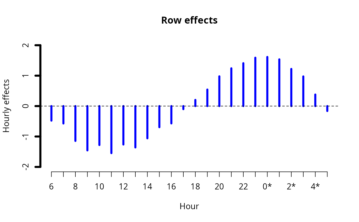
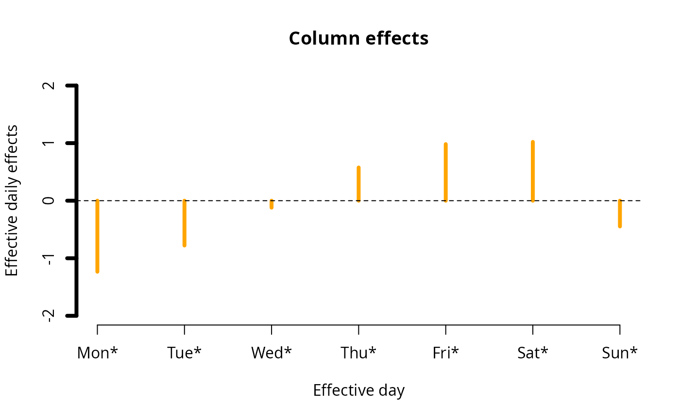
ii <- plot(fit0, rcol = "blue", ccol = "orange",
lwd = 4, ylim = c(-2, 2), # A common ylim
cylab = "Effective daily effects", rylab = "Hourly effects",
rxlab = "Hour", cxlab = "Effective day")
 ii@post # Endowed with additional information
#> $row.effects
#> [,1]
#> Row.1 -0.4781335
#> Row.2 -0.5721087
#> Row.3 -1.1449138
#> Row.4 -1.4564215
#> Row.5 -1.2800397
#> Row.6 -1.5466684
#> Row.7 -1.2631617
#> Row.8 -1.3597279
#> Row.9 -1.0594526
#> Row.10 -0.6946199
#> Row.11 -0.5700145
#> Row.12 -0.1010574
#> Row.13 0.2025315
#> Row.14 0.5431360
#> Row.15 0.9777261
#> Row.16 1.2414246
#> Row.17 1.4091096
#> Row.18 1.5897916
#> Row.19 1.6141074
#> Row.20 1.5357512
#> Row.21 1.2206984
#> Row.22 0.9746059
#> Row.23 0.3792010
#> Row.24 -0.1617638
#> attr(,"scaled:center")
#> [1] 0.4781335
#>
#> $col.effects
#> [,1]
#> Col.1 -1.2338194
#> Col.2 -0.7783439
#> Col.3 -0.1206174
#> Col.4 0.5762210
#> Col.5 0.9822999
#> Col.6 1.0214144
#> Col.7 -0.4471546
#> attr(,"scaled:center")
#> [1] 1.233819
#>
#> $raw.row.effects
#> Row.1 Row.2 Row.3 Row.4 Row.5 Row.6
#> 0.00000000 -0.09397519 -0.66678030 -0.97828796 -0.80190617 -1.06853483
#> Row.7 Row.8 Row.9 Row.10 Row.11 Row.12
#> -0.78502813 -0.88159433 -0.58131908 -0.21648637 -0.09188095 0.37707610
#> Row.13 Row.14 Row.15 Row.16 Row.17 Row.18
#> 0.68066502 1.02126950 1.45585959 1.71955808 1.88724312 2.06792510
#> Row.19 Row.20 Row.21 Row.22 Row.23 Row.24
#> 2.09224096 2.01388469 1.69883194 1.45273946 0.85733456 0.31636967
#>
#> $raw.col.effects
#> Col.1 Col.2 Col.3 Col.4 Col.5 Col.6 Col.7
#> 0.0000000 0.4554755 1.1132020 1.8100404 2.2161194 2.2552339 0.7866649
#>
# \dontrun{}
# Negative binomial example
if (FALSE) { # \dontrun{
fit1 <- rcim(alcoff.e, negbinomial, trace = TRUE)
plot(fit1, ylim = c(-2, 2)) } # }
# Univariate normal example
fit2 <- rcim(alcoff.e, uninormal, trace = TRUE)
#> Iteration 1: loglikelihood = -1232.2968
#> Iteration 2: loglikelihood = -1168.6442
#> Iteration 3: loglikelihood = -1128.0555
#> Iteration 4: loglikelihood = -1114.4362
#> Iteration 5: loglikelihood = -1113.2052
#> Iteration 6: loglikelihood = -1113.1961
#> Iteration 7: loglikelihood = -1113.1961
if (FALSE) plot(fit2, ylim = c(-200, 400)) # \dontrun{}
# Median-polish example
if (FALSE) { # \dontrun{
fit3 <- rcim(alcoff.e, alaplace1(tau = 0.5), maxit = 1000, trace = FALSE)
plot(fit3, ylim = c(-200, 250)) } # }
# Zero-inflated Poisson example on "crashp" (no 0s in alcoff)
if (FALSE) { # \dontrun{
cbind(rowSums(crashp)) # Easy to see the data
cbind(colSums(crashp)) # Easy to see the data
fit4 <- rcim(Rcim(crashp, rbaseline = "5", cbaseline = "Sun"),
zipoissonff, trace = TRUE)
plot(fit4, ylim = c(-3, 3)) } # }
ii@post # Endowed with additional information
#> $row.effects
#> [,1]
#> Row.1 -0.4781335
#> Row.2 -0.5721087
#> Row.3 -1.1449138
#> Row.4 -1.4564215
#> Row.5 -1.2800397
#> Row.6 -1.5466684
#> Row.7 -1.2631617
#> Row.8 -1.3597279
#> Row.9 -1.0594526
#> Row.10 -0.6946199
#> Row.11 -0.5700145
#> Row.12 -0.1010574
#> Row.13 0.2025315
#> Row.14 0.5431360
#> Row.15 0.9777261
#> Row.16 1.2414246
#> Row.17 1.4091096
#> Row.18 1.5897916
#> Row.19 1.6141074
#> Row.20 1.5357512
#> Row.21 1.2206984
#> Row.22 0.9746059
#> Row.23 0.3792010
#> Row.24 -0.1617638
#> attr(,"scaled:center")
#> [1] 0.4781335
#>
#> $col.effects
#> [,1]
#> Col.1 -1.2338194
#> Col.2 -0.7783439
#> Col.3 -0.1206174
#> Col.4 0.5762210
#> Col.5 0.9822999
#> Col.6 1.0214144
#> Col.7 -0.4471546
#> attr(,"scaled:center")
#> [1] 1.233819
#>
#> $raw.row.effects
#> Row.1 Row.2 Row.3 Row.4 Row.5 Row.6
#> 0.00000000 -0.09397519 -0.66678030 -0.97828796 -0.80190617 -1.06853483
#> Row.7 Row.8 Row.9 Row.10 Row.11 Row.12
#> -0.78502813 -0.88159433 -0.58131908 -0.21648637 -0.09188095 0.37707610
#> Row.13 Row.14 Row.15 Row.16 Row.17 Row.18
#> 0.68066502 1.02126950 1.45585959 1.71955808 1.88724312 2.06792510
#> Row.19 Row.20 Row.21 Row.22 Row.23 Row.24
#> 2.09224096 2.01388469 1.69883194 1.45273946 0.85733456 0.31636967
#>
#> $raw.col.effects
#> Col.1 Col.2 Col.3 Col.4 Col.5 Col.6 Col.7
#> 0.0000000 0.4554755 1.1132020 1.8100404 2.2161194 2.2552339 0.7866649
#>
# \dontrun{}
# Negative binomial example
if (FALSE) { # \dontrun{
fit1 <- rcim(alcoff.e, negbinomial, trace = TRUE)
plot(fit1, ylim = c(-2, 2)) } # }
# Univariate normal example
fit2 <- rcim(alcoff.e, uninormal, trace = TRUE)
#> Iteration 1: loglikelihood = -1232.2968
#> Iteration 2: loglikelihood = -1168.6442
#> Iteration 3: loglikelihood = -1128.0555
#> Iteration 4: loglikelihood = -1114.4362
#> Iteration 5: loglikelihood = -1113.2052
#> Iteration 6: loglikelihood = -1113.1961
#> Iteration 7: loglikelihood = -1113.1961
if (FALSE) plot(fit2, ylim = c(-200, 400)) # \dontrun{}
# Median-polish example
if (FALSE) { # \dontrun{
fit3 <- rcim(alcoff.e, alaplace1(tau = 0.5), maxit = 1000, trace = FALSE)
plot(fit3, ylim = c(-200, 250)) } # }
# Zero-inflated Poisson example on "crashp" (no 0s in alcoff)
if (FALSE) { # \dontrun{
cbind(rowSums(crashp)) # Easy to see the data
cbind(colSums(crashp)) # Easy to see the data
fit4 <- rcim(Rcim(crashp, rbaseline = "5", cbaseline = "Sun"),
zipoissonff, trace = TRUE)
plot(fit4, ylim = c(-3, 3)) } # }