Hat Values and Regression Deletion Diagnostics

When complete, a suite of functions that can be used to compute some of the regression (leave-one-out deletion) diagnostics, for the VGLM class.

Usage

hatvalues(model, ...)
hatvaluesvlm(model, type = c("diagonal", "matrix", "centralBlocks"), ...)
hatplot(model, ...)
hatplot.vlm(model, multiplier = c(2, 3), lty = "dashed",
            xlab = "Observation", ylab = "Hat values", ylim = NULL, ...)
dfbetavlm(model, maxit.new = 1,
          trace.new = FALSE,
          smallno = 1.0e-8, ...)

Arguments

model

an R object, typically returned by vglm.

type

Character. The default is the first choice, which is a \(nM \times nM\) matrix. If type = "matrix" then the entire hat matrix is returned. If type = "centralBlocks" then \(n\) central \(M \times M\) block matrices, in matrix-band format.

multiplier

Numeric, the multiplier. The usual rule-of-thumb is that values greater than two or three times the average leverage (at least for the linear model) should be checked.

lty, xlab, ylab, ylim

Graphical parameters, see par etc. The default of ylim is c(0, max(hatvalues(model))) which means that if the horizontal dashed lines cannot be seen then there are no particularly influential observations.

maxit.new, trace.new, smallno

Having maxit.new = 1 will give a one IRLS step approximation from the ordinary solution (and no warnings!). Else having maxit.new = 10, say, should usually mean convergence will occur for all observations when they are removed one-at-a-time. Else having maxit.new = 2, say, should usually mean some lack of convergence will occur when observations are removed one-at-a-time. Setting trace.new = TRUE will produce some running output at each IRLS iteration and for each individual row of the model matrix. The argument smallno multiplies each value of the original prior weight (often unity); setting it identically to zero will result in an error, but setting a very small value effectively removes that observation.

...

further arguments, for example, graphical parameters for hatplot.vlm().

Details

The invocation hatvalues(vglmObject) should return a \(n \times M\) matrix of the diagonal elements of the hat (projection) matrix of a vglm object. To do this, the QR decomposition of the object is retrieved or reconstructed, and then straightforward calculations are performed.

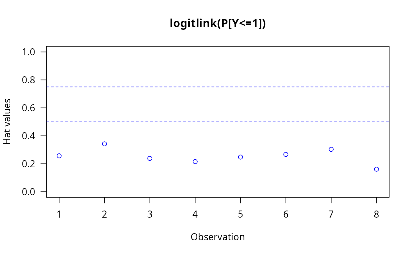
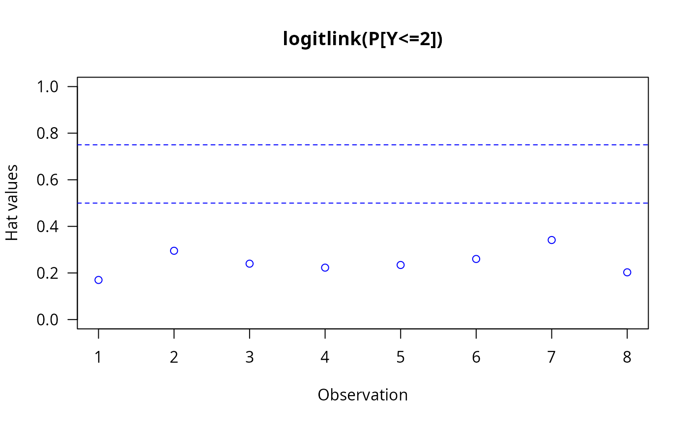
The invocation hatplot(vglmObject) should plot the diagonal of the hat matrix for each of the \(M\) linear/additive predictors. By default, two horizontal dashed lines are added; hat values higher than these ought to be checked.

Note

It is hoped, soon, that the full suite of functions described at influence.measures will be written for VGLMs. This will enable general regression deletion diagnostics to be available for the entire VGLM class.

Author

T. W. Yee.

Examples

# Proportional odds model, p.179, in McCullagh and Nelder (1989)
pneumo <- transform(pneumo, let = log(exposure.time))
fit <- vglm(cbind(normal, mild, severe) ~ let, cumulative, data = pneumo)
hatvalues(fit)  # n x M matrix, with positive values
#>   logitlink(P[Y<=1]) logitlink(P[Y<=2])
#> 1          0.2569868          0.1700224
#> 2          0.3424524          0.2952981
#> 3          0.2386174          0.2398881
#> 4          0.2154987          0.2228574
#> 5          0.2480763          0.2342776
#> 6          0.2668986          0.2601074
#> 7          0.3034072          0.3414842
#> 8          0.1613736          0.2027538
#> attr(,"predictors.names")
#> [1] "logitlink(P[Y<=1])" "logitlink(P[Y<=2])"
#> attr(,"ncol.X.vlm")
#> [1] 4
all.equal(sum(hatvalues(fit)), fit@rank)  # Should be TRUE
#> [1] TRUE
if (FALSE)  par(mfrow = c(1, 2))
hatplot(fit, ylim = c(0, 1), las = 1, col = "blue")  # \dontrun{}