Bivariate Logistic Distribution

Density, distribution function, quantile function and random generation for the 4-parameter bivariate logistic distribution.

Usage

dbilogis(x1, x2, loc1 = 0, scale1 = 1, loc2 = 0, scale2 = 1,
         log = FALSE)
pbilogis(q1, q2, loc1 = 0, scale1 = 1, loc2 = 0, scale2 = 1)
rbilogis(n, loc1 = 0, scale1 = 1, loc2 = 0, scale2 = 1)

Arguments

x1, x2, q1, q2

vector of quantiles.

n

number of observations. Same as rlogis.

loc1, loc2

the location parameters \(l_1\) and \(l_2\).

scale1, scale2

the scale parameters \(s_1\) and \(s_2\).

log

Logical. If log = TRUE then the logarithm of the density is returned.

Value

dbilogis gives the density, pbilogis gives the distribution function, and rbilogis generates random deviates (a two-column matrix).

References

Gumbel, E. J. (1961). Bivariate logistic distributions. Journal of the American Statistical Association, 56, 335–349.

Author

T. W. Yee

Details

See bilogis, the VGAM family function for estimating the four parameters by maximum likelihood estimation, for the formula of the cumulative distribution function and other details.

Note

Gumbel (1961) proposed two bivariate logistic distributions with logistic distribution marginals, which he called Type I and Type II. The Type I is this one. The Type II belongs to the Morgenstern type. The biamhcop distribution has, as a special case, this distribution, which is when the random variables are independent.

Examples

if (FALSE)  par(mfrow = c(1, 3))
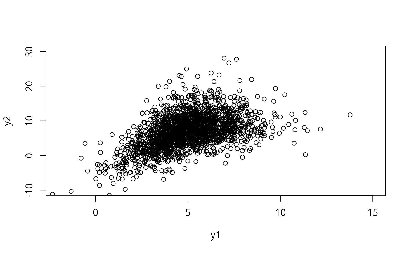
ymat <- rbilogis(n = 2000, loc1 = 5, loc2 = 7, scale2 = exp(1))
myxlim <- c(-2, 15); myylim <- c(-10, 30)
plot(ymat, xlim = myxlim, ylim = myylim)


N <- 100
x1 <- seq(myxlim[1], myxlim[2], len = N)
x2 <- seq(myylim[1], myylim[2], len = N)
ox <- expand.grid(x1, x2)
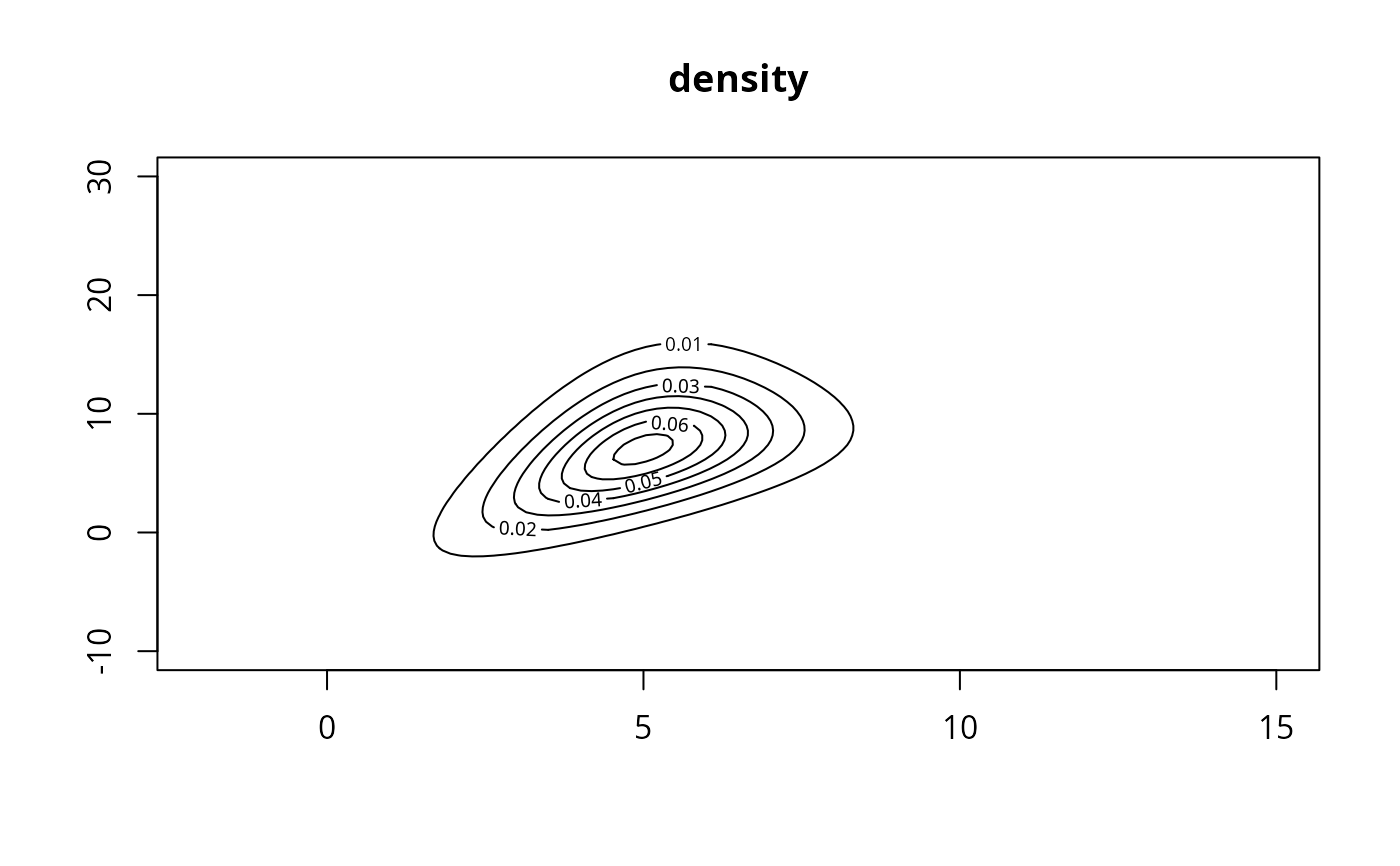
z <- dbilogis(ox[,1], ox[,2], loc1 = 5, loc2 = 7, scale2 = exp(1))
contour(x1, x2, matrix(z, N, N), main = "density")

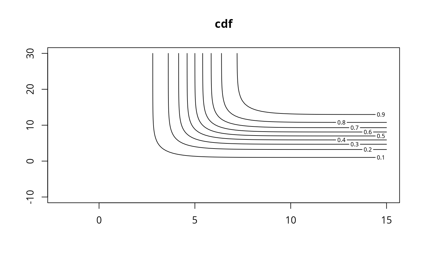
z <- pbilogis(ox[,1], ox[,2], loc1 = 5, loc2 = 7, scale2 = exp(1))
contour(x1, x2, matrix(z, N, N), main = "cdf")  # \dontrun{}