Clayton Copula (Bivariate) Distribution

Density and random generation for the (one parameter) bivariate Clayton copula distribution.

Usage

dbiclaytoncop(x1, x2, apar = 0, log = FALSE)
rbiclaytoncop(n, apar = 0)

Arguments

x1, x2

vector of quantiles. The x1 and x2 should both be in the interval \((0,1)\).

n

number of observations. Same as rnorm.

apar

the association parameter. Should be in the interval \([0, \infty)\). The default corresponds to independence.

log

Logical. If TRUE then the logarithm is returned.

Value

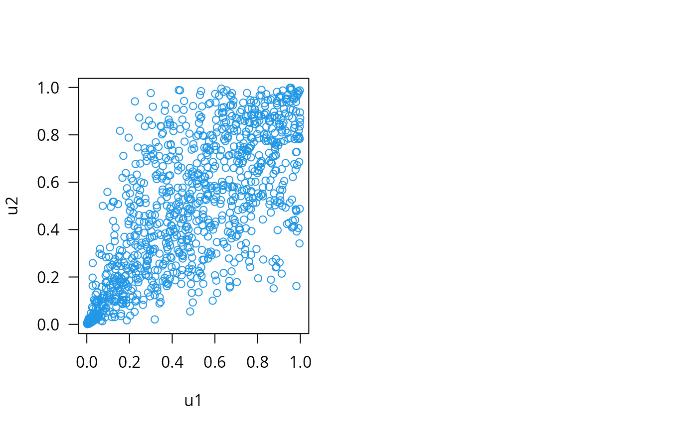
dbiclaytoncop gives the density at point (x1,x2), rbiclaytoncop generates random deviates (a two-column matrix).

References

Clayton, D. (1982). A model for association in bivariate survival data. Journal of the Royal Statistical Society, Series B, Methodological, 44, 414–422.

Author

R. Feyter and T. W. Yee

Details

See biclaytoncop, the VGAM family functions for estimating the parameter by maximum likelihood estimation, for the formula of the cumulative distribution function and other details.

Note

dbiclaytoncop() does not yet handle x1 = 0 and/or x2 = 0.

See also

biclaytoncop, binormalcop, binormal.

Examples

if (FALSE)  edge <- 0.01  # A small positive value
N <- 101; x <- seq(edge, 1.0 - edge, len = N); Rho <- 0.7
#> Error: object 'edge' not found
ox <- expand.grid(x, x)
#> Error: object 'x' not found
zedd <- dbiclaytoncop(ox[, 1], ox[, 2], apar = Rho, log = TRUE)
#> Error: object 'ox' not found
par(mfrow = c(1, 2))
contour(x, x, matrix(zedd, N, N), col = 4, labcex = 1.5, las = 1)
#> Error: object 'x' not found
plot(rbiclaytoncop(1000, 2), col = 4, las = 1)   # \dontrun{}