Outliers data

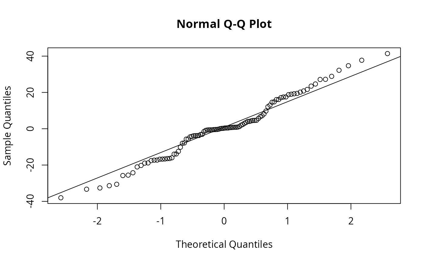
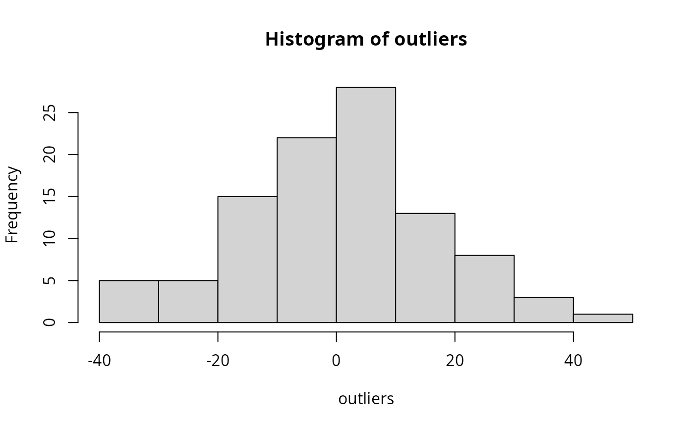
This dataset is approximately bell shaped, but with some outliers. It is meant to be used for demonstration purposes. If students are tempted to throw out all outliers, then have them work with this data (or use a scaled/centered/shuffled version as errors in a regression problem) and see how many throw away 3/4 of the data before rethinking their strategy.

data(outliers)

Format

The format is: num [1:100] -1.548 0.172 -0.638 0.233 -0.228 ...

Details

This is simulated data meant to demonstrate "outliers".

Source

Simulated, see the examples section.

Examples

data(outliers)
qqnorm(outliers)
qqline(outliers)

hist(outliers)


o.chuck <- function(x) {  # function to throw away outliers
  qq <- quantile(x, c(1,3)/4, names=FALSE)
  r <- diff(qq) * 1.5
  tst <- x < qq[1] - r | x > qq[2] + r
  if(any(tst)) {
    cat('Removing ', paste(x[tst], collapse=', '), '\n')
    x <- x[!tst]
    out <- Recall(x)
  } else {
    out <- x
  }
  out
}

x <- o.chuck( outliers )
#> Removing  -38.0188470520892, 41.3998761630706 
#> Removing  37.7254590518428 
#> Removing  -32.617721056949, 34.7123828196885, -33.3173386701734 
#> Removing  -30.5897598576629, -31.3666838246065, 32.2045826847981 
#> Removing  -25.7792864466526, 28.8645653266685 
#> Removing  -25.5510450110133, 27.1310262012897, 27.2200556465563 
#> Removing  -24.2465147302268, 24.6533216159894 
#> Removing  -21.0247217967932, 23.4707729629435 
#> Removing  20.1533689283997, 21.6405669647568, -20.2171851949336, 20.8010219332559 
#> Removing  19.2641800976782, 19.0013586098618, 18.7616896977341, 19.457788375338, -18.8293239848544, -18.9437702752492 
#> Removing  17.530663157418, 17.148643517833, 17.4680712209061, -17.268238994146, -17.3201673776458, -17.5384160660842 
#> Removing  -15.9924647726683, 16.0548292023337, -16.3808896481785, 16.1103064916208, -16.648796575613, -16.4504844329899, -16.7398192623181, -16.8005148185563 
#> Removing  -13.8846170350603, 14.5899851932271, -13.9943191858823, 14.8025506681819 
#> Removing  -12.489787807559, 13.0077936620969 
#> Removing  -10.1881202676564, 12.114181708785 
#> Removing  -7.82792554259193, -8.00899605308949, 9.73686423081927 
#> Removing  8.13154010665404 
#> Removing  -5.72028441291228, -5.7026701005752, 7.1332010769708 
#> Removing  6.5934127371113 
#> Removing  -4.50871071033652, 5.60745401739877 
#> Removing  -3.79409383578585, 4.55653891000088, -3.82862237780094, -4.21014222590597, 4.58832966905574, -3.72496986013893, 4.65320297619834, -3.89352522213875 
#> Removing  4.05151352045196, -3.17976890362346, 3.43609572821794, -3.04709006951779, 4.0309149972316, 4.33018518245162 
#> Removing  2.96065350034087 
length(x)
#> [1] 25

if(require(MASS)) {
  char2seed('robust')
  x <- 1:100
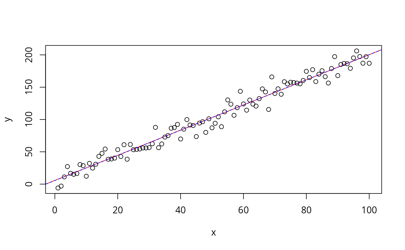
  y <- 3 + 2*x + sample(scale(outliers))*10

  plot(x,y)
  fit <- lm(y~x)
  abline(fit, col='red')

  fit.r <- rlm(y~x)
  abline(fit.r, col='blue', lty='dashed')

  rbind(coef(fit), coef(fit.r))
  length(o.chuck(resid(fit)))
}
#> Loading required package: MASS

#> Removing  25.8775509543776 
#> Removing  23.1101877518972 
#> [1] 98



### The data was generated using code similar to:

char2seed('outlier')

outliers <- rnorm(25)

dir <- 1

while( length(outliers) < 100 ){
  qq <- quantile(c(outliers, dir*Inf), c(1,3)/4)
  outliers <- c(outliers,
    qq[ 1.5 + dir/2 ] + dir*1.55*diff(qq) + dir*abs(rnorm(1)) )
  dir <- -dir
}