Periodic returns in a bar chart with risk metric overlay
Source:R/chart.BarVaR.R, R/charts.BarVaR.R
chart.BarVaR.RdPlots the periodic returns as a bar chart overlayed with a risk metric calculation.
Usage
chart.BarVaR(
  R,
  width = 0,
  gap = 12,
  methods = c("none", "ModifiedVaR", "GaussianVaR", "HistoricalVaR", "StdDev",
    "ModifiedES", "GaussianES", "HistoricalES"),
  p = 0.95,
  clean = c("none", "boudt", "geltner"),
  all = FALSE,
  ...,
  show.clean = FALSE,
  show.horizontal = FALSE,
  show.symmetric = FALSE,
  show.endvalue = FALSE,
  show.greenredbars = FALSE,
  legend.loc = "bottomleft",
  ylim = NA,
  lwd = 2,
  colorset = 1:12,
  lty = c(1, 2, 4, 5, 6),
  ypad = 0,
  legend.cex = 0.8,
  plot.engine = "default"
)

charts.BarVaR(
  R,
  main = "Returns",
  cex.legend = 0.8,
  colorset = 1:12,
  ylim = NA,
  ...,
  perpanel = NULL,
  show.yaxis = c("all", "firstonly", "alternating", "none")
)
Arguments
- R
an xts, vector, matrix, data frame, timeSeries or zoo object of asset returns
- width
periods specified for rolling-period calculations. Note that VaR, ES, and Std Dev with width=0 are calculated from the start of the timeseries
- gap
numeric number of periods from start of series to use to train risk calculation
- methods
Used to select the risk parameter of trailing
widthreturns to use: May be any of:none - does not add a risk line,
ModifiedVaR - uses Cornish-Fisher modified VaR,
GaussianVaR - uses traditional Value at Risk,
HistoricalVaR - calculates historical Value at Risk,
ModifiedES - uses Cornish-Fisher modified Expected Shortfall,
GaussianES - uses traditional Expected Shortfall,
HistoricalES - calculates historical Expected Shortfall,
StdDev - per-period standard deviation
- p
confidence level for
VaRorModifiedVaRcalculation, default is .99- clean
the method to use to clean outliers from return data prior to risk metric estimation. See
Return.cleanandVaRfor more detail- all
if TRUE, calculates risk lines for each column given in R. If FALSE, only calculates the risk line for the first column
- ...
any other passthru parameters to
chart.TimeSeries- show.clean
if TRUE and a method for 'clean' is specified, overlays the actual data with the "cleaned" data. See
Return.cleanfor more detail- show.horizontal
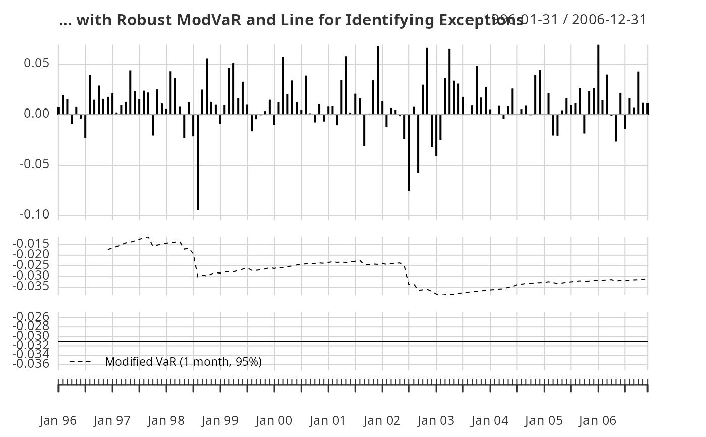
if TRUE, shows a line across the timeseries at the value of the most recent VaR estimate, to help the reader evaluate the number of exceptions thus far
- show.symmetric
if TRUE and the metric is symmetric, this will show the metric's positive values as well as negative values, such as for method "StdDev".
- show.endvalue
if TRUE, show the final (out of sample) value
- show.greenredbars
if TRUE, show the per-period returns using green and red bars for positive and negative returns
- legend.loc
legend location, such as in
chart.TimeSeries- ylim
set the y-axis limit, same as in
plot- lwd
set the line width, same as in
plot- colorset
color palette to use, such as in
chart.TimeSeries- lty
set the line type, same as in
plot- ypad
adds a numerical padding to the y-axis to keep the data away when legend.loc="bottom". See examples below.
- legend.cex
sets the legend text size, such as in
chart.TimeSeries- plot.engine
Choose the engine for plotting, including "default","dygraph","ggplot","plotly" and "googleVis"
- main
sets the title text, such as in
chart.TimeSeries- cex.legend
sets the legend text size, such as in
chart.TimeSeries- perpanel
default NULL, controls column display
- show.yaxis
one of "all", "firstonly", "alternating", or "none" to control where y axis is plotted in multipanel charts
Details
Note that StdDev and VaR are symmetric calculations, so a high
and low measure will be plotted. ModifiedVaR, on the other hand, is
assymetric and only a lower bound will be drawn.
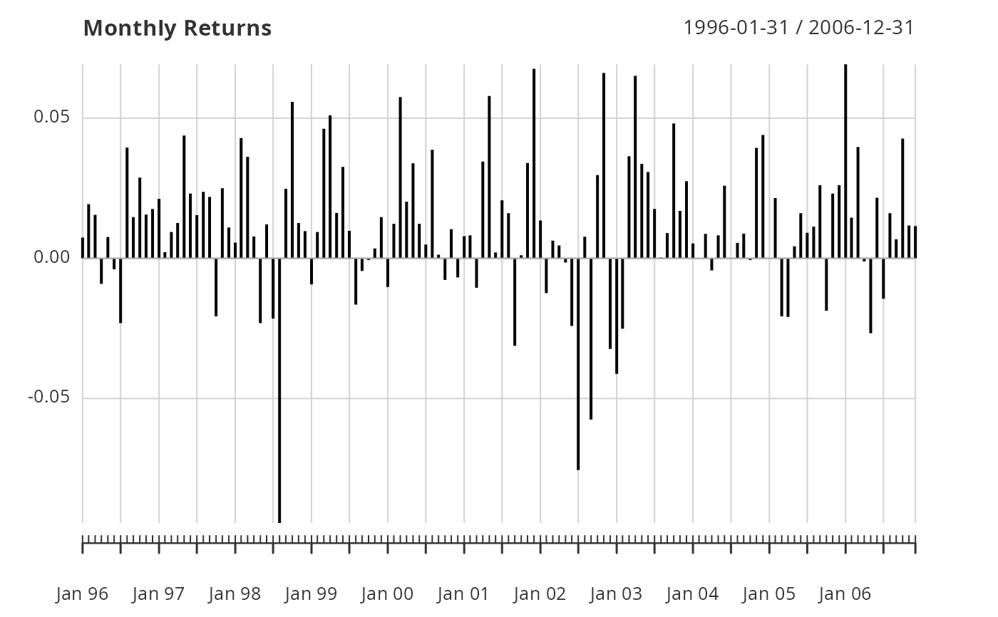
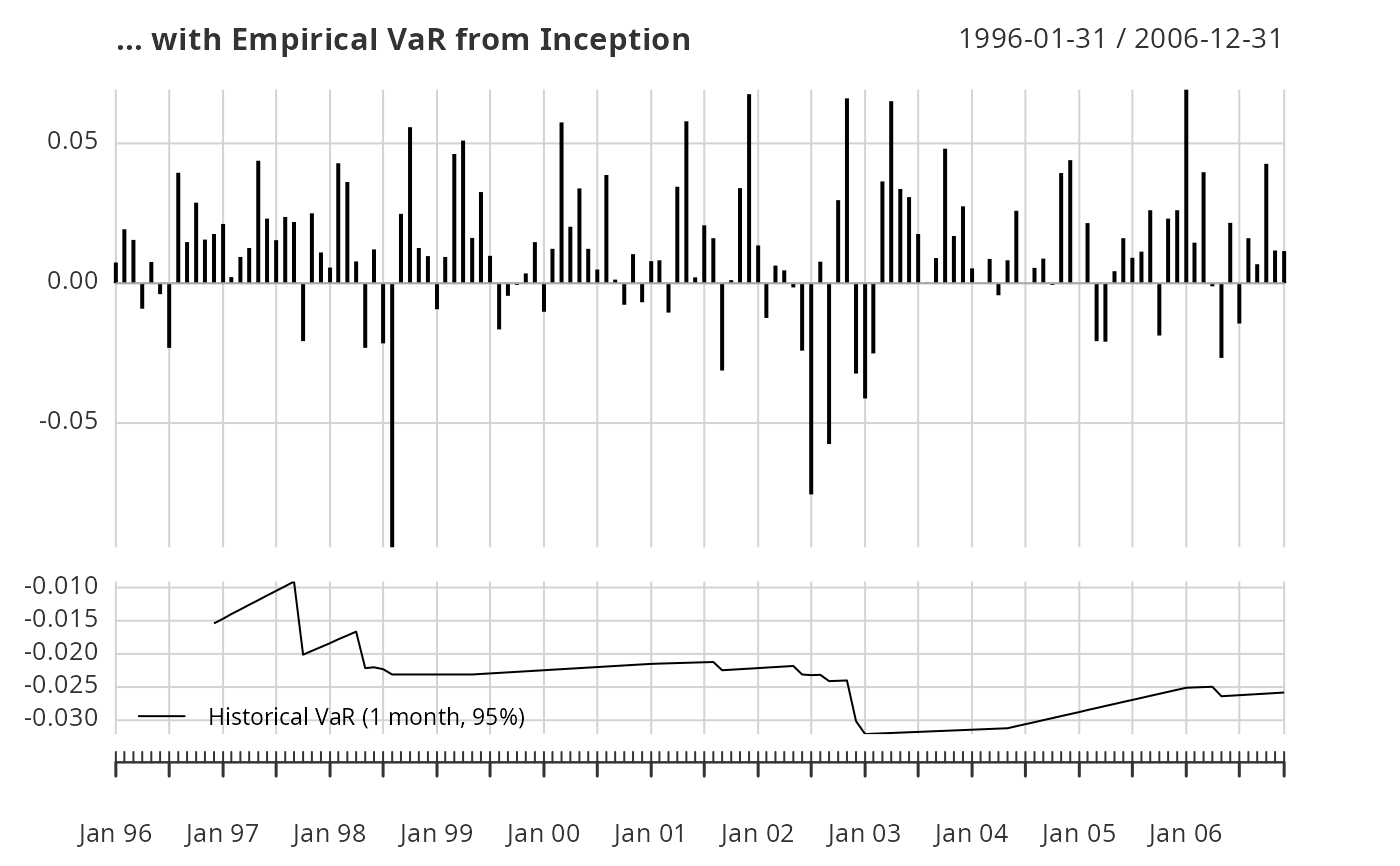
Creates a plot of time on the x-axis and vertical lines for each period to indicate value on the y-axis. Overlays a line to indicate the value of a risk metric calculated at that time period.
charts.BarVaR places multile bar charts in a single
graphic, with associated risk measures
Examples
if (FALSE) # not run on CRAN because of example time
data(managers)
# plain
chart.BarVaR(managers[,1,drop=FALSE], main="Monthly Returns")
 # with risk line
chart.BarVaR(managers[,1,drop=FALSE],
methods="HistoricalVaR",
main="... with Empirical VaR from Inception")
# with risk line
chart.BarVaR(managers[,1,drop=FALSE],
methods="HistoricalVaR",
main="... with Empirical VaR from Inception")
 # with lines for all managers in the sample
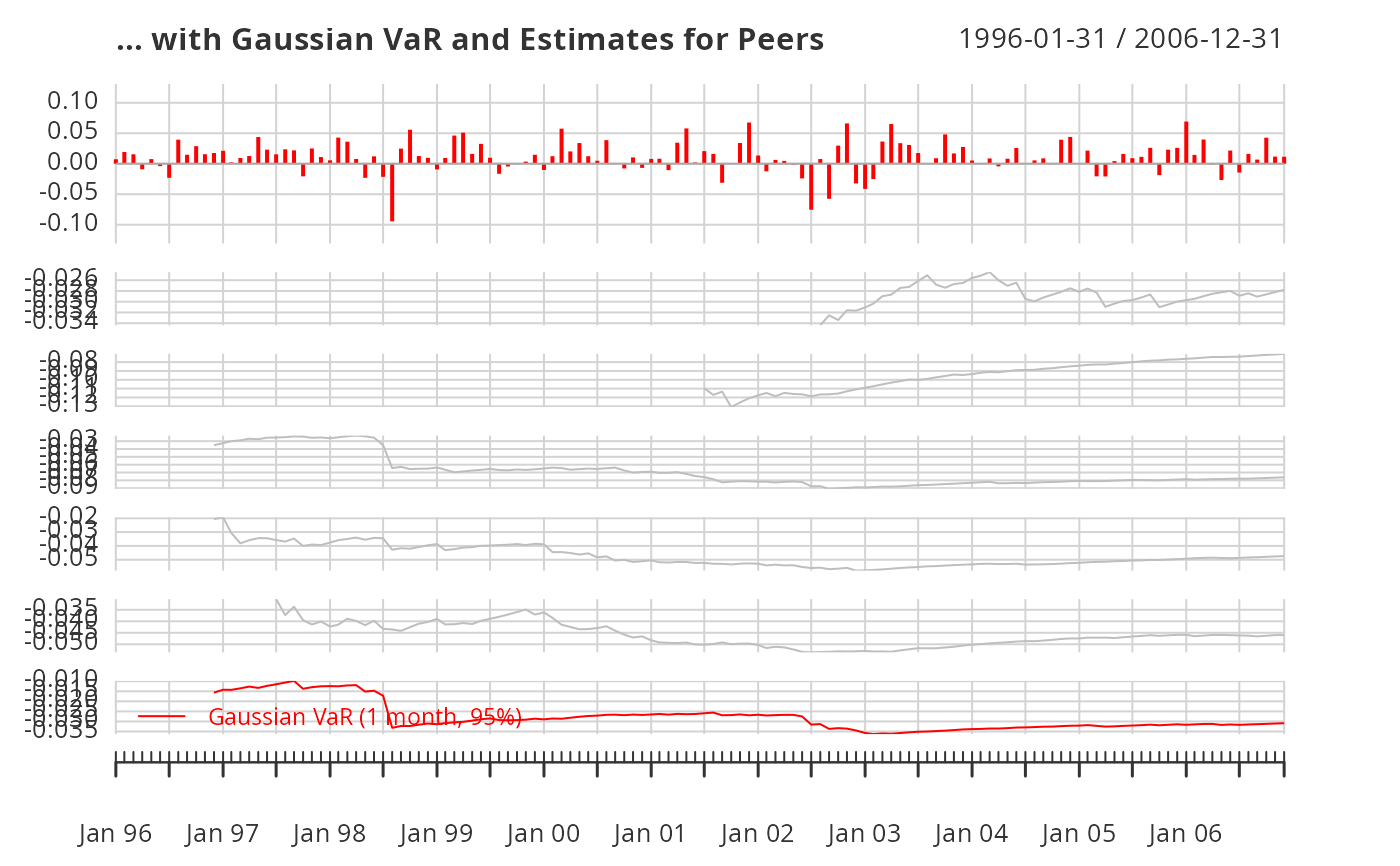
chart.BarVaR(managers[,1:6],
methods="GaussianVaR",
all=TRUE, lty=1, lwd=2,
colorset= c("red", rep("gray", 5)),
main="... with Gaussian VaR and Estimates for Peers")
# with lines for all managers in the sample
chart.BarVaR(managers[,1:6],
methods="GaussianVaR",
all=TRUE, lty=1, lwd=2,
colorset= c("red", rep("gray", 5)),
main="... with Gaussian VaR and Estimates for Peers")
 # with multiple methods
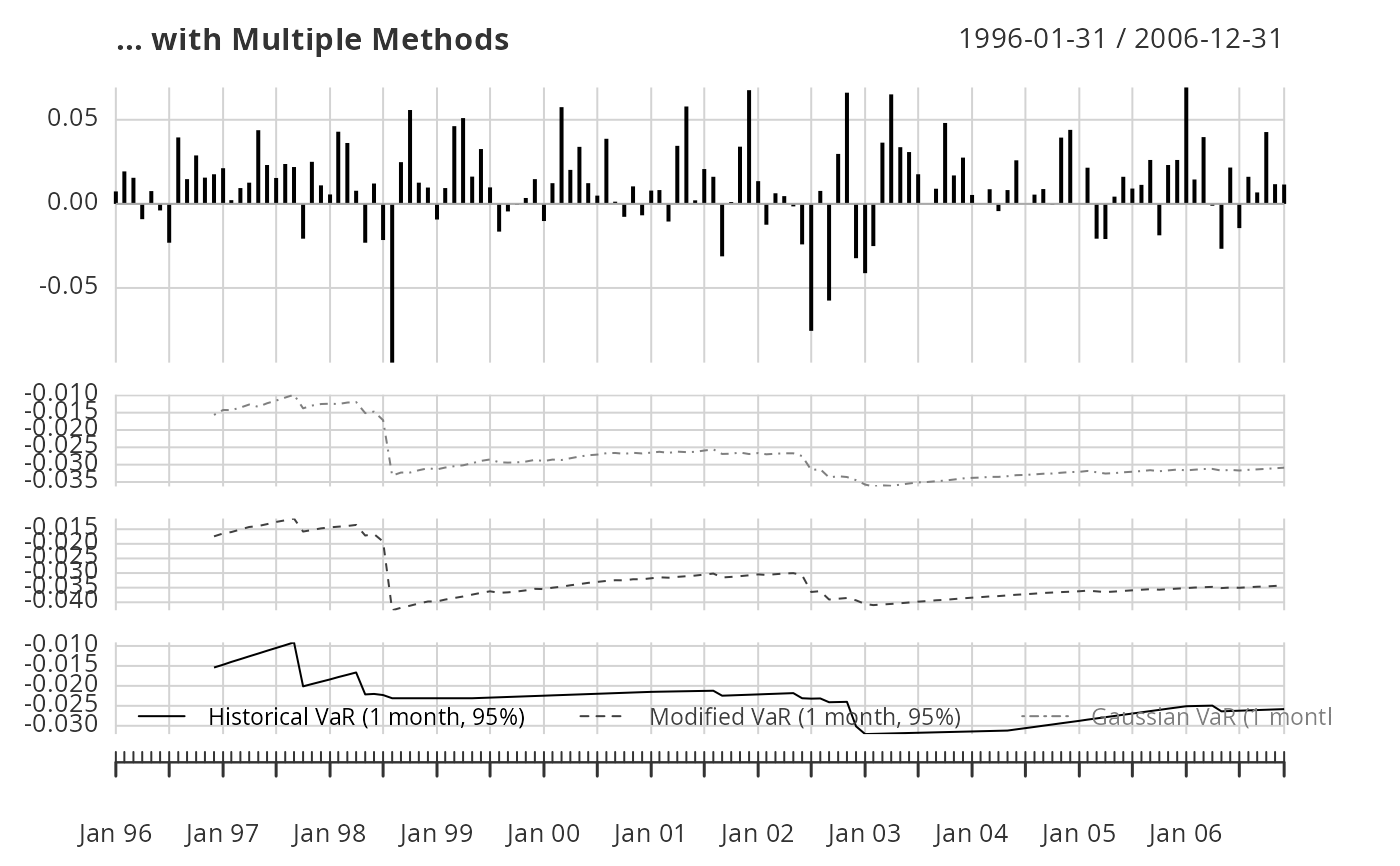
chart.BarVaR(managers[,1,drop=FALSE],
methods=c("HistoricalVaR", "ModifiedVaR", "GaussianVaR"),
main="... with Multiple Methods")
# with multiple methods
chart.BarVaR(managers[,1,drop=FALSE],
methods=c("HistoricalVaR", "ModifiedVaR", "GaussianVaR"),
main="... with Multiple Methods")
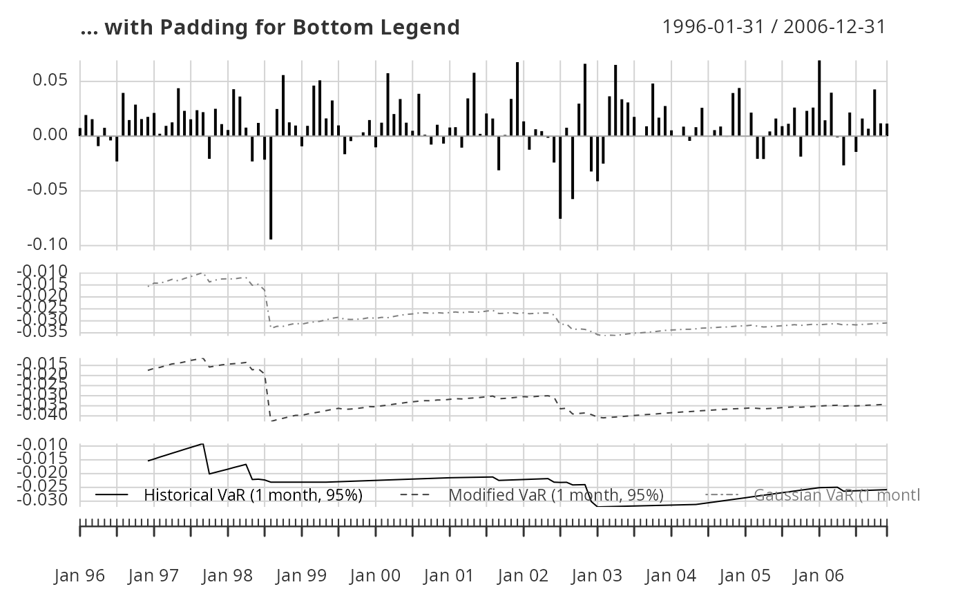
 # cleaned up a bit
chart.BarVaR(managers[,1,drop=FALSE],
methods=c("HistoricalVaR", "ModifiedVaR", "GaussianVaR"),
lwd=2, ypad=.01,
main="... with Padding for Bottom Legend")
# cleaned up a bit
chart.BarVaR(managers[,1,drop=FALSE],
methods=c("HistoricalVaR", "ModifiedVaR", "GaussianVaR"),
lwd=2, ypad=.01,
main="... with Padding for Bottom Legend")
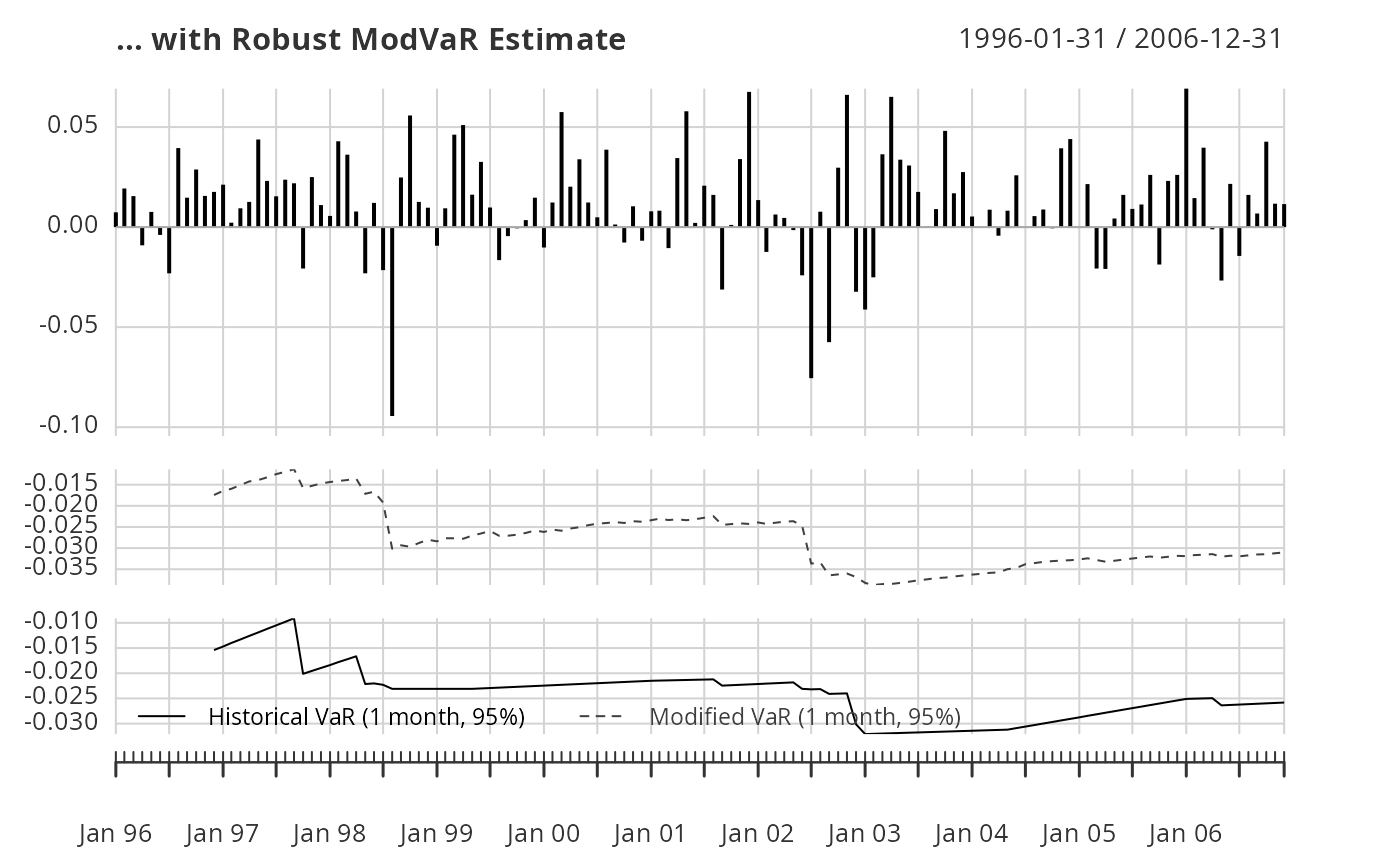
 # with 'cleaned' data for VaR estimates
chart.BarVaR(managers[,1,drop=FALSE],
methods=c("HistoricalVaR", "ModifiedVaR"),
lwd=2, ypad=.01, clean="boudt",
main="... with Robust ModVaR Estimate")
# with 'cleaned' data for VaR estimates
chart.BarVaR(managers[,1,drop=FALSE],
methods=c("HistoricalVaR", "ModifiedVaR"),
lwd=2, ypad=.01, clean="boudt",
main="... with Robust ModVaR Estimate")
 # Cornish Fisher VaR estimated with cleaned data,
# with horizontal line to show exceptions
chart.BarVaR(managers[,1,drop=FALSE],
methods="ModifiedVaR",
lwd=2, ypad=.01, clean="boudt",
show.horizontal=TRUE, lty=2,
main="... with Robust ModVaR and Line for Identifying Exceptions")
# Cornish Fisher VaR estimated with cleaned data,
# with horizontal line to show exceptions
chart.BarVaR(managers[,1,drop=FALSE],
methods="ModifiedVaR",
lwd=2, ypad=.01, clean="boudt",
show.horizontal=TRUE, lty=2,
main="... with Robust ModVaR and Line for Identifying Exceptions")
 # \dontrun{}