Higher Moments Summary: Statistics and Stylized Facts

Summary of the higher moements and Co-Moments of the return distribution. Used to determine diversification potential. Also called "systematic" moments by several papers.

table.HigherMoments(Ra, Rb, scale = NA, Rf = 0, digits = 4, method = "moment")

Arguments

Ra

an xts, vector, matrix, data frame, timeSeries or zoo object of asset returns

Rb

return vector of the benchmark asset

scale

number of periods in a year (daily scale = 252, monthly scale = 12, quarterly scale = 4)

Rf

risk free rate, in same period as your returns

digits

number of digits to round results to

method

method to use when computing kurtosis one of: excess, moment, fisher

References

Martellini L., Vaissie M., Ziemann V. Investing in Hedge Funds: Adding Value through Active Style Allocation Decisions. October 2005. Edhec Risk and Asset Management Research Centre.

See also

CoSkewness
CoKurtosis
BetaCoVariance
BetaCoSkewness
BetaCoKurtosis
skewness
kurtosis

Author

Peter Carl

Examples

data(managers)
table.HigherMoments(managers[,1:3],managers[,8,drop=FALSE])
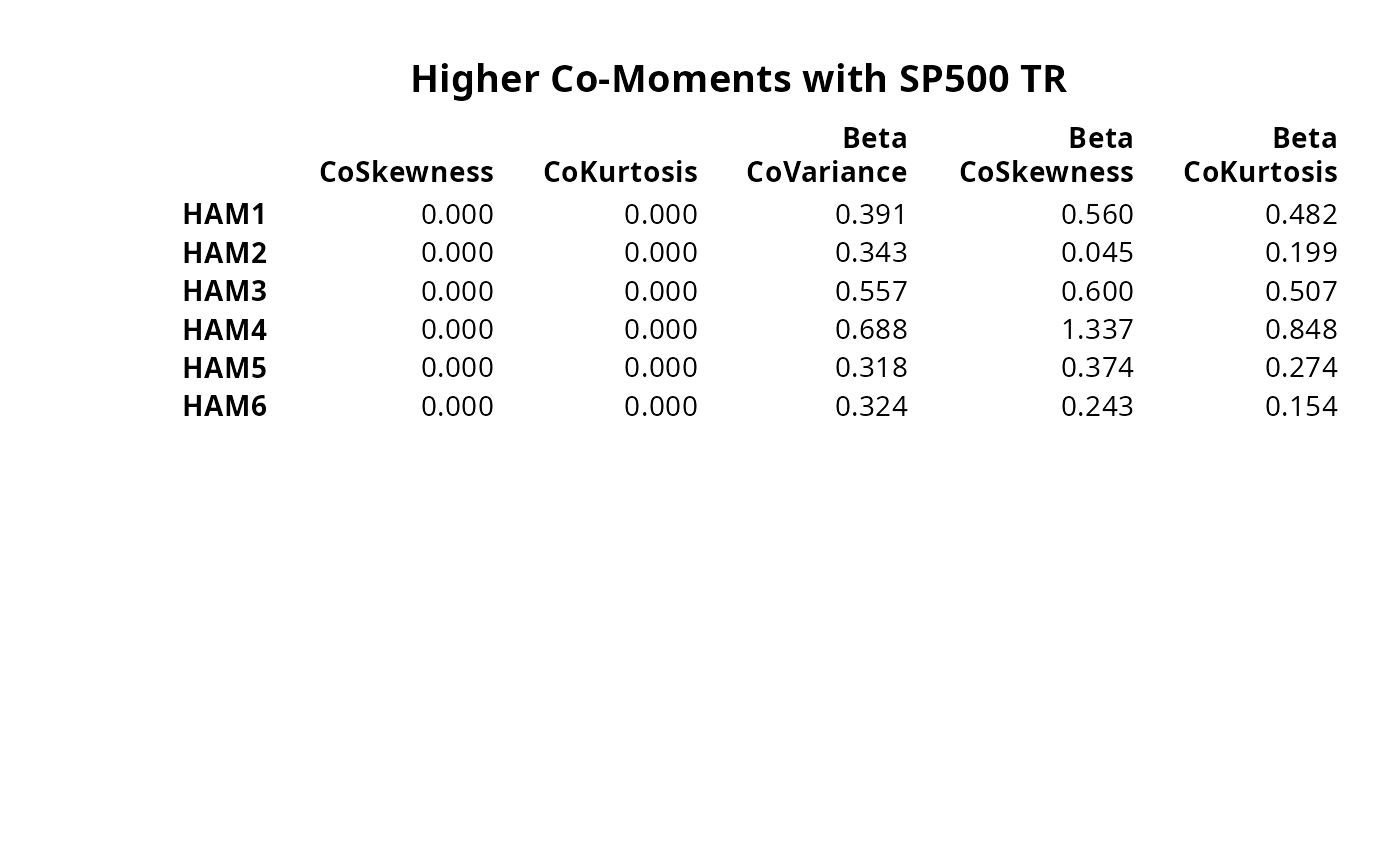
#>                 HAM1 to SP500 TR HAM2 to SP500 TR HAM3 to SP500 TR
#> CoSkewness                0.0000           0.0000           0.0000
#> CoKurtosis                0.0000           0.0000           0.0000
#> Beta CoVariance           0.3906           0.3432           0.5572
#> Beta CoSkewness           0.5602           0.0454           0.5999
#> Beta CoKurtosis           0.4815           0.1988           0.5068
result=t(table.HigherMoments(managers[,1:6],managers[,8,drop=FALSE]))
rownames(result)=colnames(managers[,1:6])

 # don't test on CRAN, since it requires Suggested packages

require("Hmisc")
textplot(format.df(result, na.blank=TRUE, numeric.dollar=FALSE, 
         cdec=rep(3,dim(result)[2])), rmar = 0.8, cmar = 1.5,  
         max.cex=.9, halign = "center", valign = "top", row.valign="center", 
         wrap.rownames=5, wrap.colnames=10, mar = c(0,0,3,0)+0.1)
title(main="Higher Co-Moments with SP500 TR")