Functions for calculating the nearest comoment estimator for financial time series

calculates NCE covariance, coskewness and cokurtosis matrices

MM.NCE(R, as.mat = TRUE, ...)

Arguments

R

an xts, vector, matrix, data frame, timeSeries or zoo object of asset returns (with mean zero)

as.mat

TRUE/FALSE whether to return the full moment matrix or only the vector with the unique elements (the latter is advised for speed), default TRUE

...

any other passthru parameters, see details.

Details

The coskewness and cokurtosis matrices are defined as the matrices of dimension p x p^2 and p x p^3 containing the third and fourth order central moments. They are useful for measuring nonlinear dependence between different assets of the portfolio and computing modified VaR and modified ES of a portfolio.

The nearest comoment estimator is a way to estimate the covariance, coskewness and cokurtosis matrix by means of a latent multi-factor model. The method is proposed in Boudt, Cornilly and Verdonck (2018).

The optional arguments include the number of factors, given by `k` and the weight matrix `W`, see the examples.

References

Boudt, Kris, Dries Cornilly and Tim Verdonck. 2020. Nearest comoment estimation with unobserved factors. Journal of Econometrics, 217(2), 381-397.

See also

CoMoments
ShrinkageMoments
StructuredMoments
EWMAMoments
MCA

Author

Dries Cornilly

Examples

if (FALSE)  # CRAN doesn't like how long this takes (>5 secs)
data(edhec)

# default estimator
est_nc <- MM.NCE(edhec[, 1:3] * 100)

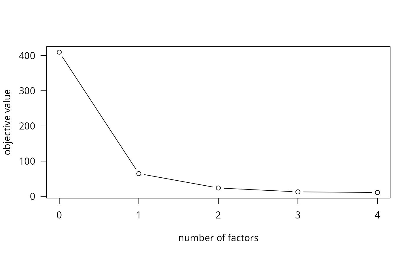
# scree plot to determine number of factors
obj <- rep(NA, 5)
for (ii in 1:5) {
    est_nc <- MM.NCE(edhec[, 1:5] * 100, k = ii - 1)
    obj[ii] <- est_nc$optim.sol$objective * nrow(edhec[, 1:5])
}
plot(0:4, obj, type = 'b', xlab = "number of factors", 
     ylab = "objective value", las = 1)

     
# bootstrapped estimator
est_nc <- MM.NCE(edhec[, 1:2] * 100, W = list("Wid" = "RidgeD",
                 "alpha" = NULL, "nb" = 250, "alphavec" = seq(0.2, 1, by = 0.2)))
                 
# ridge weight matrix with alpha = 0.5
est_nc <- MM.NCE(edhec[, 1:2] * 100, W = list("Wid" = "RidgeD", "alpha" = 0.5))
 # \dontrun{} # end \dontrun