The formal model underlying the procedure is based on a so called functional relationship: $$x_i=\xi_i + e_{1i}, \qquad y_i=\alpha + \beta \xi_i + e_{2i}$$ with \(\mathrm{var}(e_{1i})=\sigma\), \(\mathrm{var}(e_{2i})=\lambda\sigma\), where \(\lambda\) is the known variance ratio.
Deming(
  x,
  y,
  vr = sdr^2,
  sdr = sqrt(vr),
  boot = FALSE,
  keep.boot = FALSE,
  alpha = 0.05
)
Arguments
- x
a numeric variable
- y
a numeric variable
- vr
The assumed known ratio of the (residual) variance of the
ys relative to that of thexs. Defaults to 1.- sdr
do. for standard deviations. Defaults to 1.
vrtakes precedence if both are given.- boot
Should bootstrap estimates of standard errors of parameters be done? If
boot==TRUE, 1000 bootstrap samples are done, ifbootis numeric,bootsamples are made.- keep.boot
Should the 4-column matrix of bootstrap samples be returned? If
TRUE, the summary is printed, but the matrix is returned invisibly. Ignored ifboot=FALSE- alpha
What significance level should be used when displaying confidence intervals?
Value
If boot==FALSE a named vector with components
Intercept, Slope, sigma.x, sigma.y, where x
and y are substituted by the variable names.
If boot==TRUE a matrix with rows Intercept,
Slope, sigma.x, sigma.y, and colums giving the estimates,
the bootstrap standard error and the bootstrap estimate and c.i. as the 0.5,
\(\alpha/2\) and \(1-\alpha/2\) quantiles of the sample.
If keep.boot==TRUE this summary is printed, but a matrix with columns
Intercept,
Slope, sigma.x, sigma.y and boot rows is returned.
Details
The estimates of the residual variance is based on a weighting of the sum of squared deviations in both directions, divided by \(n-2\). The ML estimate would use \(2n\) instead, but in the model we actually estimate \(n+2\) parameters — \(\alpha, \beta\) and the \(n\) \(\xi s\). This is not in Peter Sprent's book (see references).
References
Peter Sprent: Models in Regression, Methuen & Co., London 1969, ch.3.4.
WE Deming: Statistical adjustment of data, New York: Wiley, 1943.
Examples
# 'True' values
M <- runif(100,0,5)
# Measurements:
x <- M + rnorm(100)
y <- 2 + 3 * M + rnorm(100,sd=2)
# Deming regression with equal variances, variance ratio 2.
Deming(x,y)
#> Intercept Slope sigma.x sigma.y
#> 0.4225056 3.4461777 1.0608452 1.0608452
Deming(x,y,vr=2)
#> Intercept Slope sigma.x sigma.y
#> 0.8577821 3.2813864 1.0202102 1.4427951
Deming(x,y,boot=TRUE)
#> y = alpha + beta* x
#> Estimate S.e.(boot) 50% 2.5% 97.5%
#> Intercept 0.4225056 0.99409089 0.3901545 -1.6022482 2.182090
#> Slope 3.4461777 0.31373390 3.4565645 2.8902761 4.102815
#> sigma.x 1.0608452 0.07265842 1.0502534 0.9024009 1.188907
#> sigma.y 1.0608452 0.07265842 1.0502534 0.9024009 1.188907
bb <- Deming(x,y,boot=TRUE,keep.boot=TRUE)
#> Estimate S.e.(boot) 50% 2.5% 97.5%
#> Intercept 0.4225056 0.95366623 0.4631722 -1.4791399 2.144844
#> Slope 3.4461777 0.30038548 3.4539047 2.8900721 4.070234
#> sigma.x 1.0608452 0.07105165 1.0461995 0.9122294 1.182947
#> sigma.y 1.0608452 0.07105165 1.0461995 0.9122294 1.182947
str(bb)
#> num [1:1000, 1:4] 0.444 0.941 0.119 1.196 2.05 ...
#> - attr(*, "dimnames")=List of 2
#> ..$ : NULL
#> ..$ : chr [1:4] "Intercept" "Slope" "sigma.x" "sigma.y"
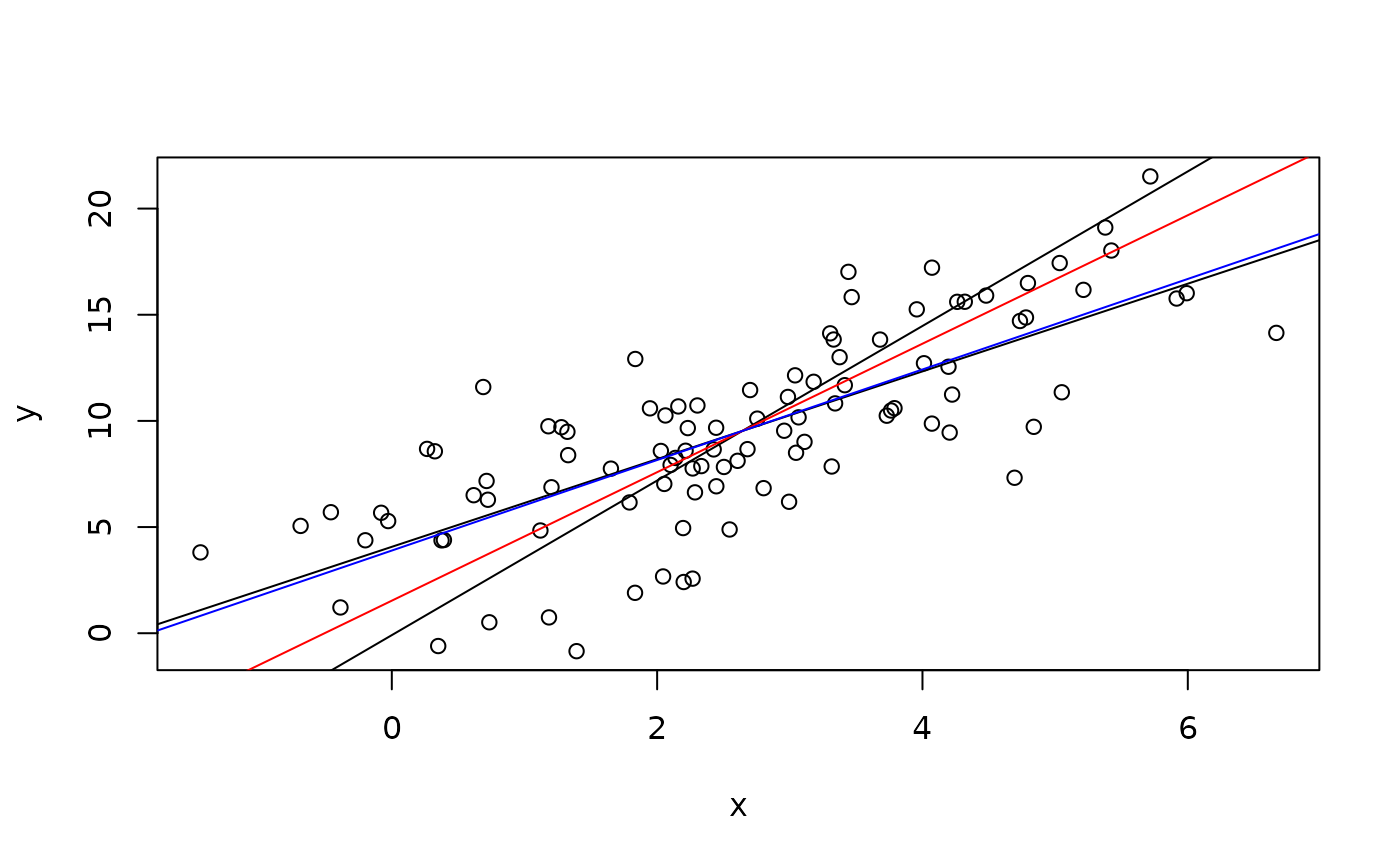
# Plot data with the two classical regression lines
plot(x,y)
abline(lm(y~x))
ir <- coef(lm(x~y))
abline(-ir[1]/ir[2],1/ir[2])
abline(Deming(x,y,sdr=2)[1:2],col="red")
abline(Deming(x,y,sdr=10)[1:2],col="blue")
 # Comparing classical regression and "Deming extreme"
summary(lm(y~x))
#>
#> Call:
#> lm(formula = y ~ x)
#>
#> Residuals:
#> Min 1Q Median 3Q Max
#> -7.7910 -1.5459 0.3227 2.2214 6.1036
#>
#> Coefficients:
#> Estimate Std. Error t value Pr(>|t|)
#> (Intercept) 4.0691 0.5682 7.161 1.49e-10 ***
#> x 2.0656 0.1822 11.339 < 2e-16 ***
#> ---
#> Signif. codes: 0 ‘***’ 0.001 ‘**’ 0.01 ‘*’ 0.05 ‘.’ 0.1 ‘ ’ 1
#>
#> Residual standard error: 3.023 on 98 degrees of freedom
#> Multiple R-squared: 0.5675, Adjusted R-squared: 0.5631
#> F-statistic: 128.6 on 1 and 98 DF, p-value: < 2.2e-16
#>
Deming(x,y,vr=1000000)
#> Intercept Slope sigma.x sigma.y
#> 4.069033430 2.065639654 0.003022665 3.022664824
# Comparing classical regression and "Deming extreme"
summary(lm(y~x))
#>
#> Call:
#> lm(formula = y ~ x)
#>
#> Residuals:
#> Min 1Q Median 3Q Max
#> -7.7910 -1.5459 0.3227 2.2214 6.1036
#>
#> Coefficients:
#> Estimate Std. Error t value Pr(>|t|)
#> (Intercept) 4.0691 0.5682 7.161 1.49e-10 ***
#> x 2.0656 0.1822 11.339 < 2e-16 ***
#> ---
#> Signif. codes: 0 ‘***’ 0.001 ‘**’ 0.01 ‘*’ 0.05 ‘.’ 0.1 ‘ ’ 1
#>
#> Residual standard error: 3.023 on 98 degrees of freedom
#> Multiple R-squared: 0.5675, Adjusted R-squared: 0.5631
#> F-statistic: 128.6 on 1 and 98 DF, p-value: < 2.2e-16
#>
Deming(x,y,vr=1000000)
#> Intercept Slope sigma.x sigma.y
#> 4.069033430 2.065639654 0.003022665 3.022664824