Two-Dimensional Kernel Density Estimation

Two-dimensional kernel density estimation with an axis-aligned bivariate normal kernel, evaluated on a square grid.

kde2d(x, y, h, n = 25, lims = c(range(x), range(y)))

Arguments

x

x coordinate of data

y

y coordinate of data

h

vector of bandwidths for x and y directions. Defaults to normal reference bandwidth (see bandwidth.nrd). A scalar value will be taken to apply to both directions.

n

Number of grid points in each direction. Can be scalar or a length-2 integer vector.

lims

The limits of the rectangle covered by the grid as c(xl, xu, yl, yu).

Value

A list of three components.

x, y

The x and y coordinates of the grid points, vectors of length n.

z

An n[1] by n[2] matrix of the estimated density: rows correspond to the value of x, columns to the value of y.

References

Venables, W. N. and Ripley, B. D. (2002) Modern Applied Statistics with S. Fourth edition. Springer.

Examples

attach(geyser)
plot(duration, waiting, xlim = c(0.5,6), ylim = c(40,100))

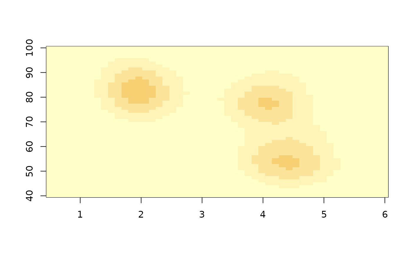
f1 <- kde2d(duration, waiting, n = 50, lims = c(0.5, 6, 40, 100))
image(f1, zlim = c(0, 0.05))

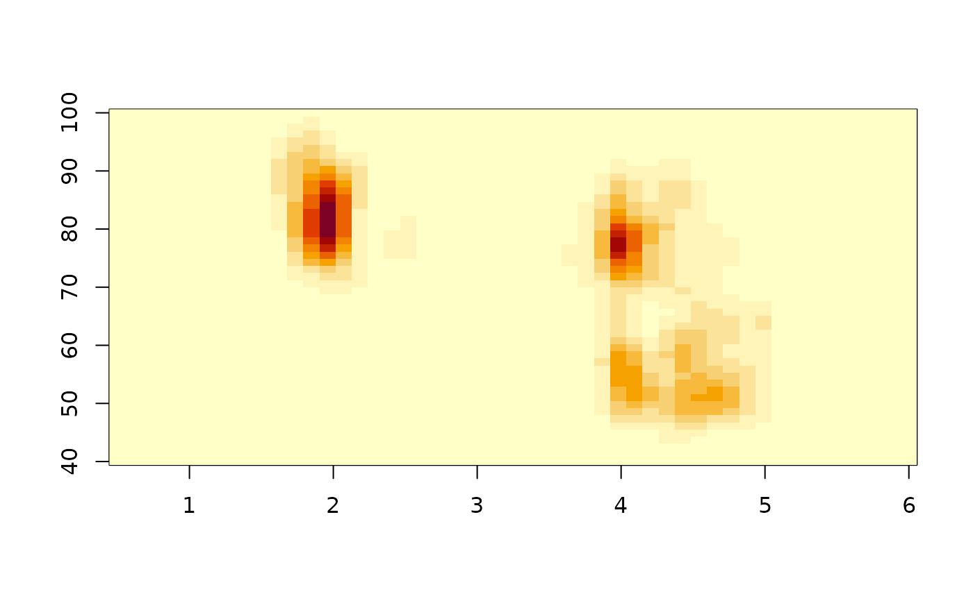
f2 <- kde2d(duration, waiting, n = 50, lims = c(0.5, 6, 40, 100),
            h = c(width.SJ(duration), width.SJ(waiting)) )
image(f2, zlim = c(0, 0.05))

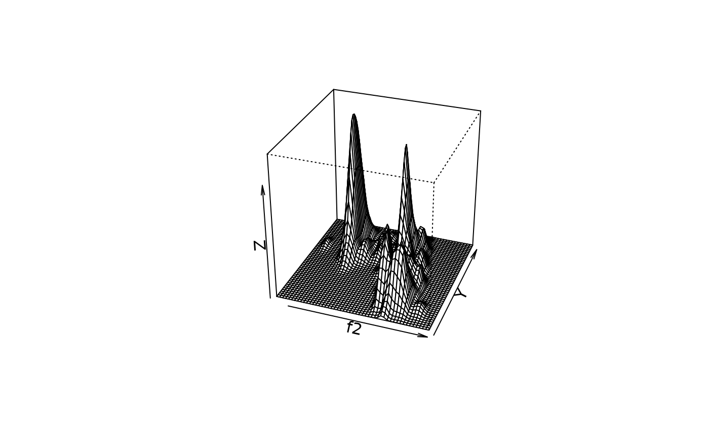
persp(f2, phi = 30, theta = 20, d = 5)


plot(duration[-272], duration[-1], xlim = c(0.5, 6),
     ylim = c(1, 6),xlab = "previous duration", ylab = "duration")

f1 <- kde2d(duration[-272], duration[-1],
            h = rep(1.5, 2), n = 50, lims = c(0.5, 6, 0.5, 6))
contour(f1, xlab = "previous duration",
        ylab = "duration", levels  =  c(0.05, 0.1, 0.2, 0.4) )

f1 <- kde2d(duration[-272], duration[-1],
            h = rep(0.6, 2), n = 50, lims = c(0.5, 6, 0.5, 6))
contour(f1, xlab = "previous duration",
        ylab = "duration", levels  =  c(0.05, 0.1, 0.2, 0.4) )

f1 <- kde2d(duration[-272], duration[-1],
            h = rep(0.4, 2), n = 50, lims = c(0.5, 6, 0.5, 6))
contour(f1, xlab = "previous duration",
        ylab = "duration", levels  =  c(0.05, 0.1, 0.2, 0.4) )

detach("geyser")