Frequency Scatterplot
ggfreqScatter.RdUses ggplot2 to plot a scatterplot or dot-like chart for the case
where there is a very large number of overlapping values. This works
for continuous and categorical x and y. For continuous
variables it serves the same purpose as hexagonal binning. Counts for
overlapping points are grouped into quantile groups and level of
transparency and rainbow colors are used to provide count information.
Instead, you can specify stick=TRUE not use color but to encode
cell frequencies
with the height of a black line y-centered at the middle of the bins.
Relative frequencies are not transformed, and the maximum cell
frequency is shown in a caption. Every point with at least a
frequency of one is depicted with a full-height light gray vertical
line, scaled to the above overall maximum frequency. In this way to
relative frequency is to proportion of these light gray lines that are
black, and one can see points whose frequencies are too low to see the
black lines.
The result can also be passed to ggplotly. Actual cell
frequencies are added to the hover text in that case using the
label ggplot2 aesthetic.
Usage
ggfreqScatter(x, y, by=NULL, bins=50, g=10, cuts=NULL,
              xtrans = function(x) x,
              ytrans = function(y) y,
              xbreaks = pretty(x, 10),
              ybreaks = pretty(y, 10),
              xminor  = NULL, yminor = NULL,
              xlab = as.character(substitute(x)),
              ylab = as.character(substitute(y)),
              fcolors = viridisLite::viridis(10), nsize=FALSE,
              stick=FALSE, html=FALSE, prfreq=FALSE, ...)
Arguments
- x
x-variable
- y
y-variable
- by
an optional vector used to make separate plots for each distinct value using
facet_wrap()- bins
for continuous
xoryis the number of bins to create by rounding. Ignored for categorical variables. If a 2-vector, the first element corresponds toxand the second toy.- g
number of quantile groups to make for frequency counts. Use
g=0to use frequencies continuously for color coding. This is recommended only when usingplotly.- cuts
instead of using
g, specifycutsto provide the vector of cuts for categorizing frequencies for assignment to colors- xtrans,ytrans
functions specifying transformations to be made before binning and plotting
- xbreaks,ybreaks
vectors of values to label on axis, on original scale
- xminor,yminor
values at which to put minor tick marks, on original scale
- xlab,ylab
axis labels. If not specified and variable has a
label, thatu label will be used.- fcolors
colorsargument to pass toscale_color_gradientnto color code frequencies. Usefcolors=gray.colors(10, 0.75, 0)to show gray scale, for example. Another good choice isfcolors=hcl.colors(10, 'Blue-Red').- nsize
set to
TRUEto not vary color or transparency but instead to size the symbols in relation to the number of points. Best with bothxandyare discrete.ggplot2sizeis taken as the fourth root of the frequency. If there are 15 or unique frequencies all the unique frequencies are used, otherwisegquantile groups of frequencies are used.- stick
set to
TRUEto not use colors but instead use varying-height black vertical lines to depict cell frequencies.- html
set to
TRUEto use html in axis labels instead of plotmath- prfreq
set to
TRUEto print the frequency distributions of the binned coordinate frequencies- ...
arguments to pass to
geom_pointsuch asshapeandsize
Examples
require(ggplot2)
set.seed(1)
x <- rnorm(1000)
y <- rnorm(1000)
count <- sample(1:100, 1000, TRUE)
x <- rep(x, count)
y <- rep(y, count)
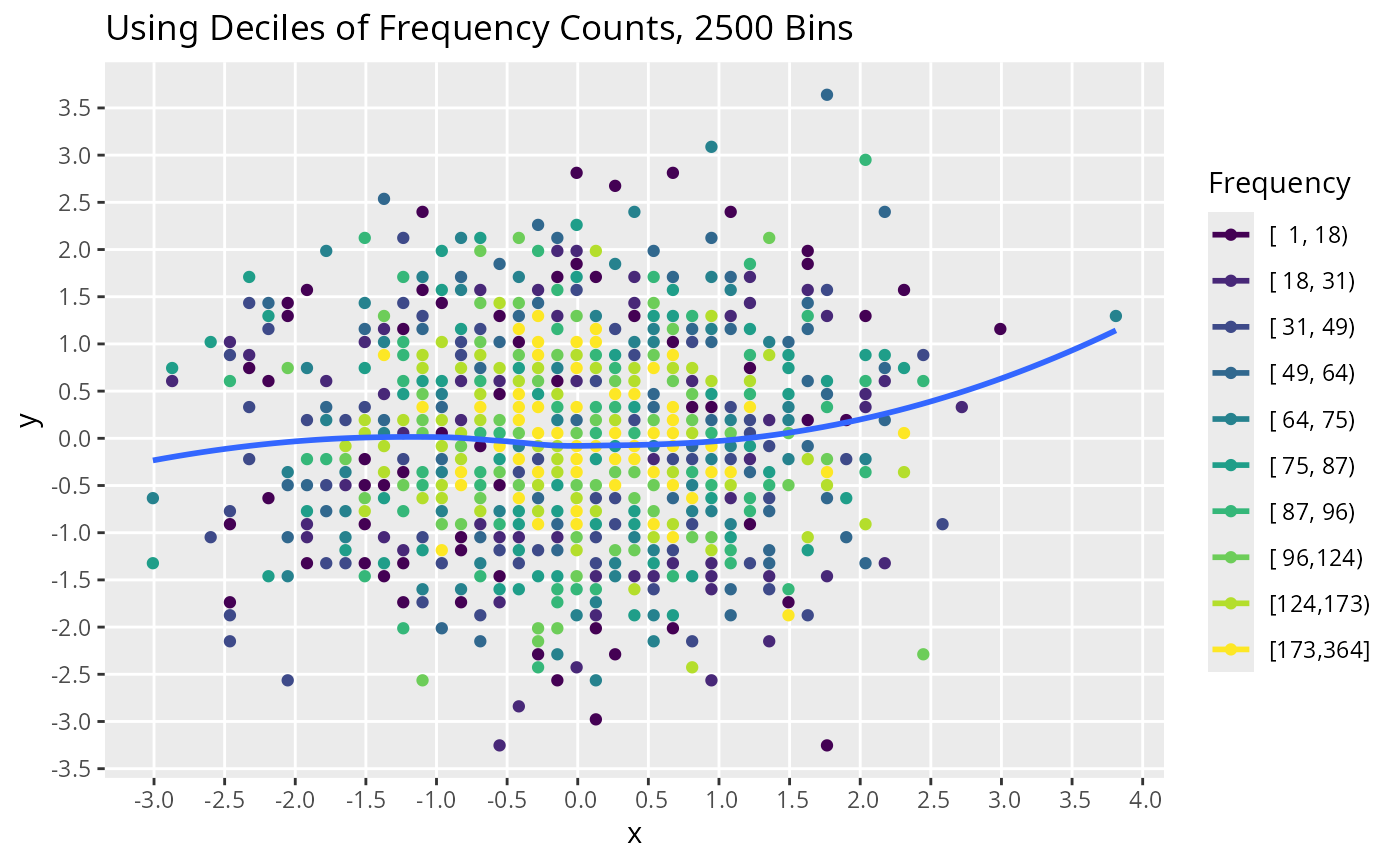
# color=alpha=NULL below makes loess smooth over all points
g <- ggfreqScatter(x, y) + # might add g=0 if using plotly
geom_smooth(aes(color=NULL, alpha=NULL), se=FALSE) +
ggtitle("Using Deciles of Frequency Counts, 2500 Bins")
g
#> `geom_smooth()` using method = 'loess' and formula = 'y ~ x'
#> Warning: The following aesthetics were dropped during statistical transformation: label.
#> ℹ This can happen when ggplot fails to infer the correct grouping structure in
#> the data.
#> ℹ Did you forget to specify a `group` aesthetic or to convert a numerical
#> variable into a factor?
 # plotly::ggplotly(g, tooltip='label') # use plotly, hover text = freq. only
# Plotly makes it somewhat interactive, with hover text tooltips
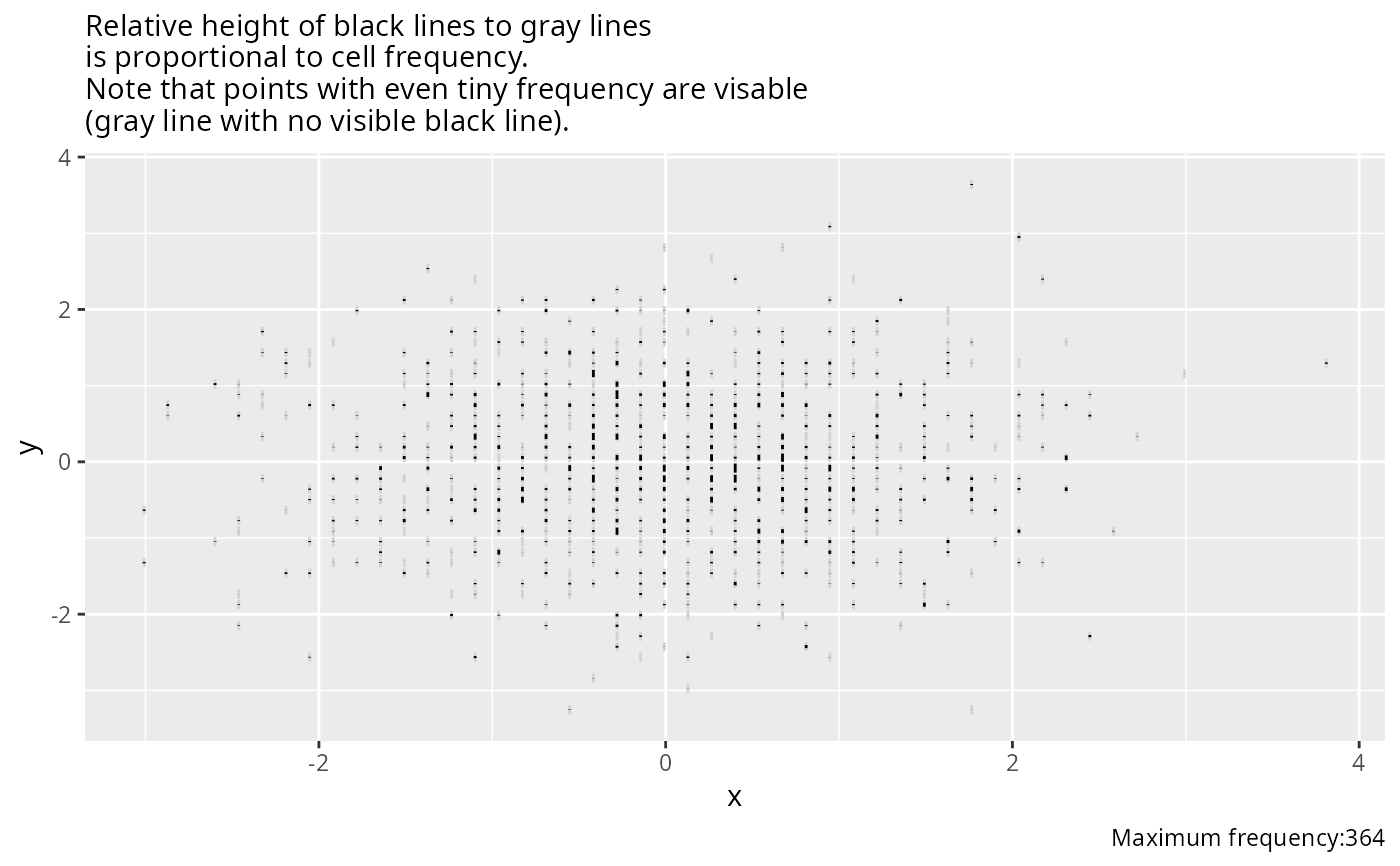
# Instead use varying-height sticks to depict frequencies
ggfreqScatter(x, y, stick=TRUE) +
labs(subtitle='Relative height of black lines to gray lines
is proportional to cell frequency.
Note that points with even tiny frequency are visable
(gray line with no visible black line).')
#> Warning: Removed 1 row containing missing values or values outside the scale range
#> (`geom_segment()`).
#> Warning: Removed 1 row containing missing values or values outside the scale range
#> (`geom_segment()`).
# plotly::ggplotly(g, tooltip='label') # use plotly, hover text = freq. only
# Plotly makes it somewhat interactive, with hover text tooltips
# Instead use varying-height sticks to depict frequencies
ggfreqScatter(x, y, stick=TRUE) +
labs(subtitle='Relative height of black lines to gray lines
is proportional to cell frequency.
Note that points with even tiny frequency are visable
(gray line with no visible black line).')
#> Warning: Removed 1 row containing missing values or values outside the scale range
#> (`geom_segment()`).
#> Warning: Removed 1 row containing missing values or values outside the scale range
#> (`geom_segment()`).
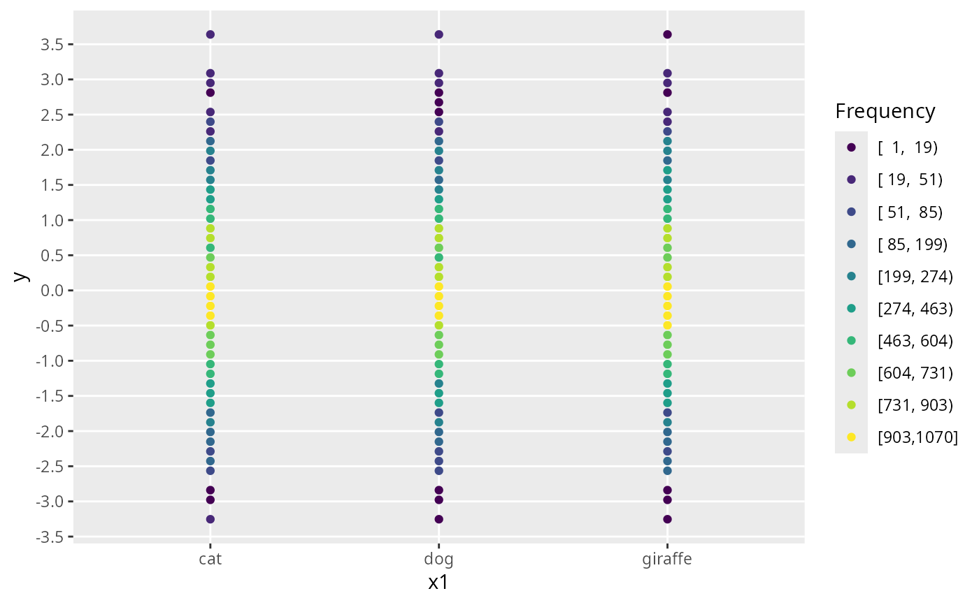
 # Try with x categorical
x1 <- sample(c('cat', 'dog', 'giraffe'), length(x), TRUE)
ggfreqScatter(x1, y)
# Try with x categorical
x1 <- sample(c('cat', 'dog', 'giraffe'), length(x), TRUE)
ggfreqScatter(x1, y)
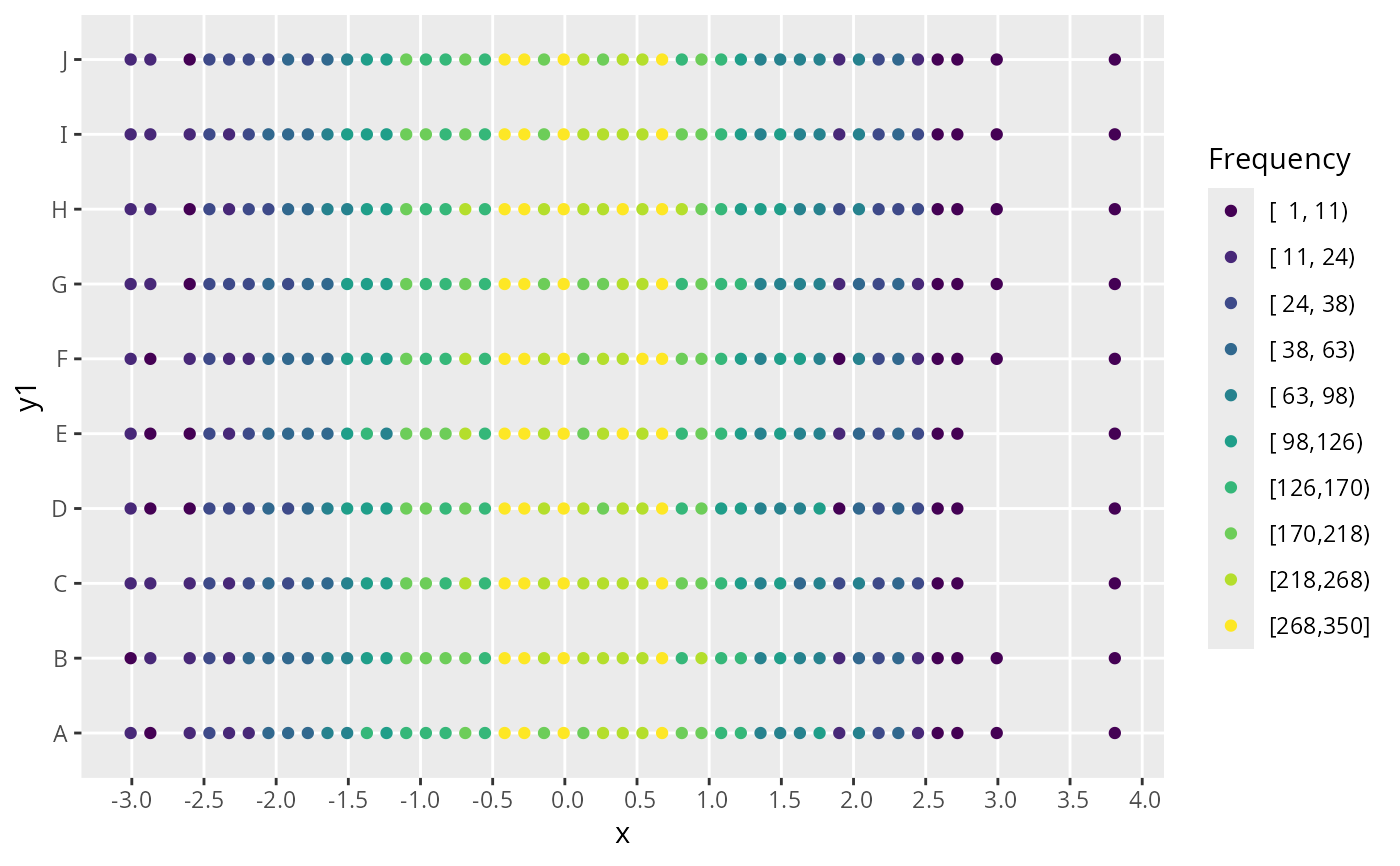
 # Try with y categorical
y1 <- sample(LETTERS[1:10], length(x), TRUE)
ggfreqScatter(x, y1)
# Try with y categorical
y1 <- sample(LETTERS[1:10], length(x), TRUE)
ggfreqScatter(x, y1)
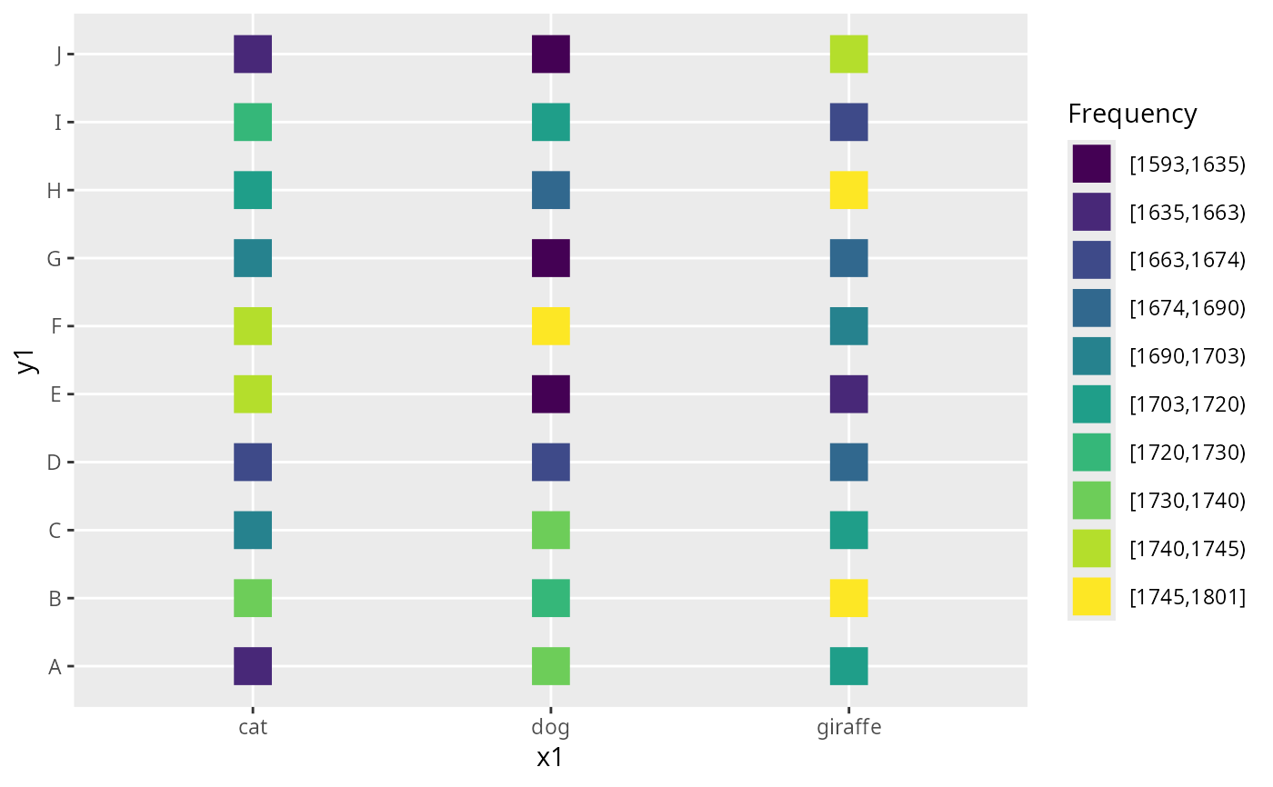
 # Both categorical, larger point symbols, box instead of circle
ggfreqScatter(x1, y1, shape=15, size=7)
# Both categorical, larger point symbols, box instead of circle
ggfreqScatter(x1, y1, shape=15, size=7)
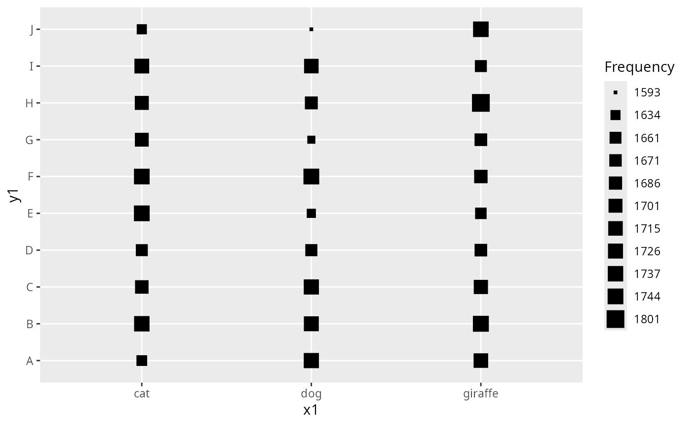
 # Vary box size instead
ggfreqScatter(x1, y1, nsize=TRUE, shape=15)
# Vary box size instead
ggfreqScatter(x1, y1, nsize=TRUE, shape=15)