Gaussian Kernel R6 class
Gaussian Kernel R6 class
Usage
k_Gaussian(
  beta,
  s2 = 1,
  D,
  beta_lower = -8,
  beta_upper = 6,
  beta_est = TRUE,
  s2_lower = 1e-08,
  s2_upper = 1e+08,
  s2_est = TRUE,
  useC = TRUE,
  isotropic = FALSE
)
Format
R6Class object.
Arguments
- beta
Initial beta value
- s2
Initial variance
- D
Number of input dimensions of data
- beta_lower
Lower bound for beta
- beta_upper
Upper bound for beta
- beta_est
Should beta be estimated?
- s2_lower
Lower bound for s2
- s2_upper
Upper bound for s2
- s2_est
Should s2 be estimated?
- useC
Should C code used? Much faster.
- isotropic
If isotropic then a single beta/theta is used for all dimensions. If not (anisotropic) then a separate beta/beta is used for each dimension.
Value
Object of R6Class with methods for fitting GP model.
Super classes
GauPro::GauPro_kernel -> GauPro::GauPro_kernel_beta -> GauPro_kernel_Gaussian
Methods
Inherited methods
GauPro::GauPro_kernel$plot()GauPro::GauPro_kernel_beta$initialize()GauPro::GauPro_kernel_beta$param_optim_lower()GauPro::GauPro_kernel_beta$param_optim_start()GauPro::GauPro_kernel_beta$param_optim_start0()GauPro::GauPro_kernel_beta$param_optim_upper()GauPro::GauPro_kernel_beta$s2_from_params()GauPro::GauPro_kernel_beta$set_params_from_optim()
Method d2C_dudv_ueqvrows()
Second derivative of covariance with respect to X and XX when they equal the same value
Examples
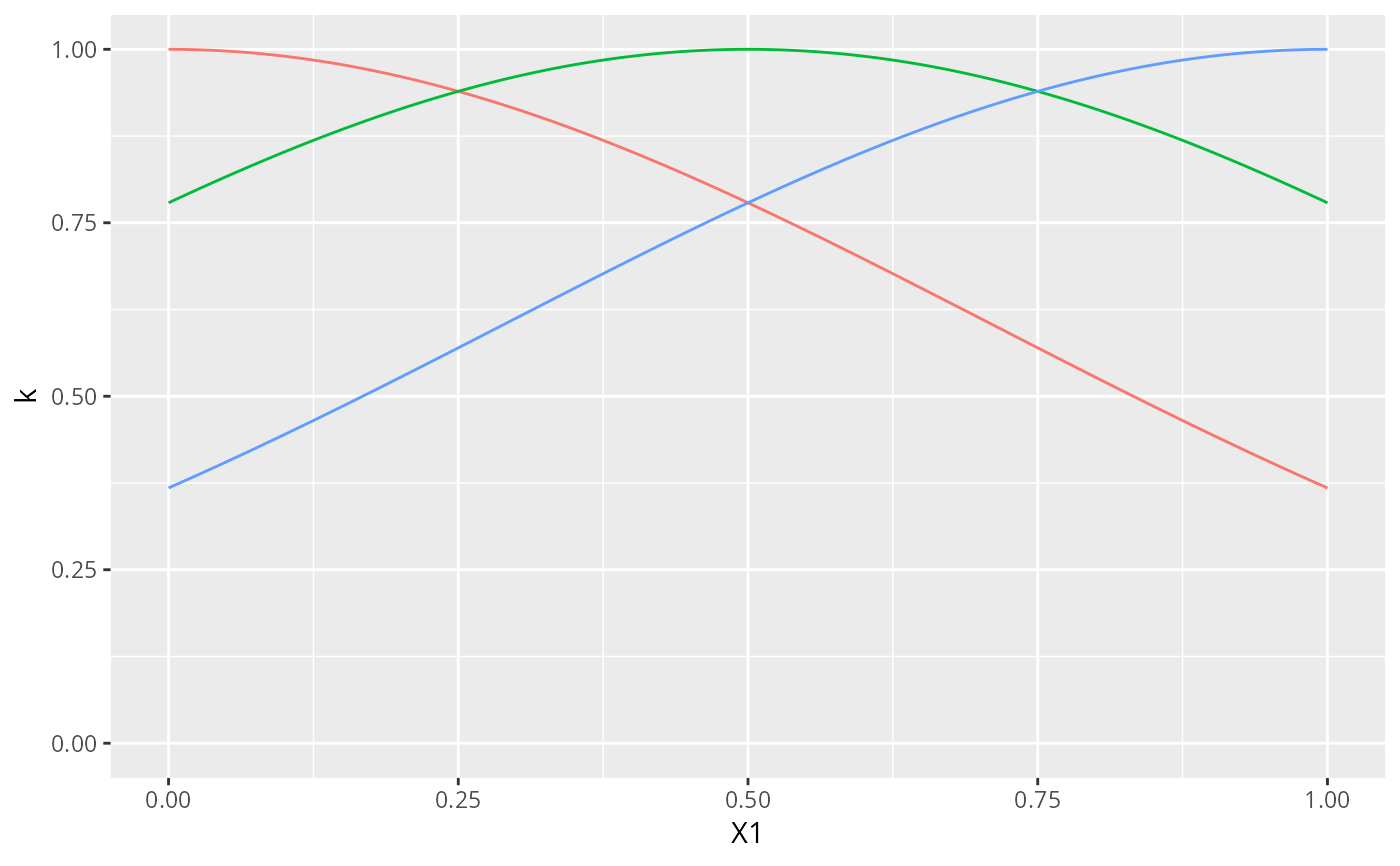
k1 <- Gaussian$new(beta=0)
plot(k1)
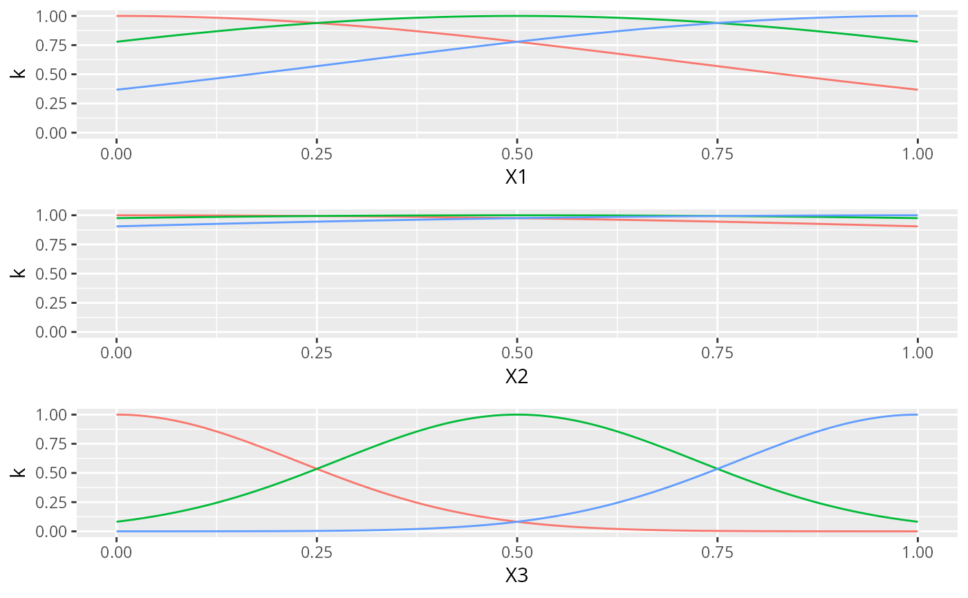
 k1 <- Gaussian$new(beta=c(0,-1, 1))
plot(k1)
k1 <- Gaussian$new(beta=c(0,-1, 1))
plot(k1)
 n <- 12
x <- matrix(seq(0,1,length.out = n), ncol=1)
y <- sin(2*pi*x) + rnorm(n,0,1e-1)
gp <- GauPro_kernel_model$new(X=x, Z=y, kernel=Gaussian$new(1),
parallel=FALSE)
#> * nug is at minimum value after optimizing. Check the fit to see it this caused a bad fit. Consider changing nug.min. This is probably fine for noiseless data.
gp$predict(.454)
#> [1] 0.3042196
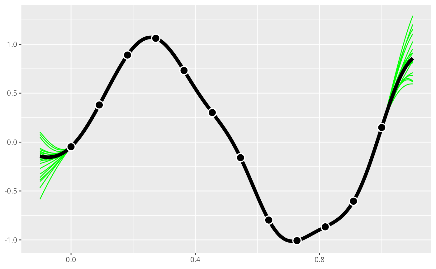
gp$plot1D()
n <- 12
x <- matrix(seq(0,1,length.out = n), ncol=1)
y <- sin(2*pi*x) + rnorm(n,0,1e-1)
gp <- GauPro_kernel_model$new(X=x, Z=y, kernel=Gaussian$new(1),
parallel=FALSE)
#> * nug is at minimum value after optimizing. Check the fit to see it this caused a bad fit. Consider changing nug.min. This is probably fine for noiseless data.
gp$predict(.454)
#> [1] 0.3042196
gp$plot1D()
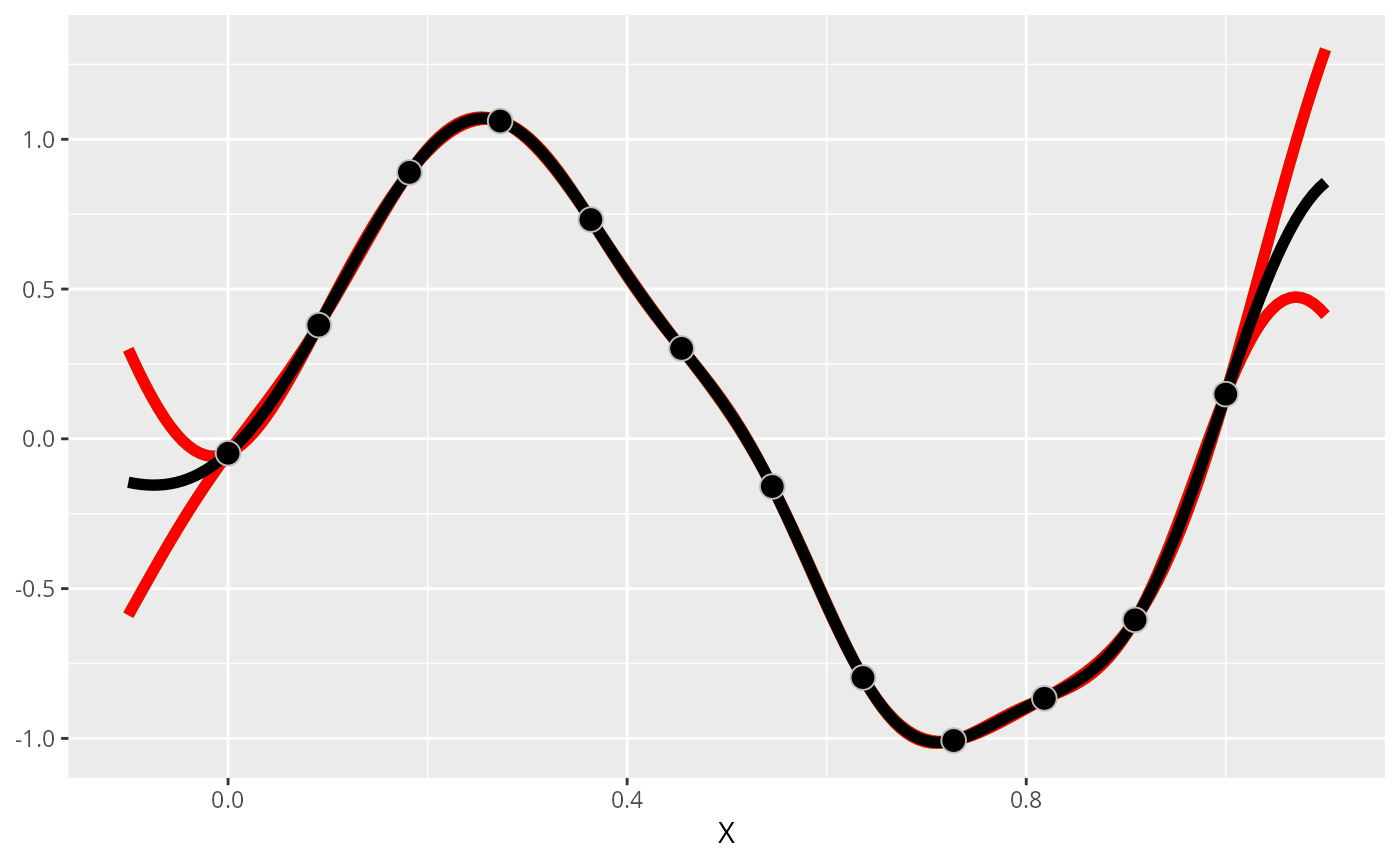 gp$cool1Dplot()