This function tests if a user-defined summary differs when applied to simulated / observed data.
Usage
testGeneric(simulationOutput, summary, alternative = c("two.sided",
  "greater", "less"), plot = T,
  methodName = "DHARMa generic simulation test")
Arguments
- simulationOutput
an object of class DHARMa, either created via simulateResiduals for supported models or by createDHARMa for simulations created outside DHARMa, or a supported model. Providing a supported model directly is discouraged, because simulation settings cannot be changed in this case.
- summary
a function that can be applied to simulated / observed data. See examples below.
- alternative
a character string specifying whether the test should test if observations are "greater", "less" or "two.sided" compared to the simulated null hypothesis.
- plot
whether to plot the simulated summary.
- methodName
name of the test (will be used in plot).
Details
This function applies a user-defined summary to the simulated / observed data of a DHARMa object and then performs a hypothesis test using the ratio Obs / Sim as the test statistic.
The summary is applied directly to the data and not to the residuals, but it can easily be remodeled to apply summaries to the residuals by simply defining something like f = function(x) summary (x - predictions), as done in testDispersion.
Note
The summary function you specify will be applied to the data as it appears in your fitted model, which may not always be what you want.
As an example, consider the case where we want to test for n-inflation in k/n data. If you provide your data via cbind (k, n-k), you have to test for n-inflation, but if you provide your data via k/n and weights = n, you should test for 1-inflation. When in doubt, check how the data is represented internally in model.frame(model) or via simulate(model).
Examples
testData = createData(sampleSize = 100, overdispersion = 0.5, randomEffectVariance = 0)
fittedModel <- glm(observedResponse ~ Environment1 , family = "poisson", data = testData)
simulationOutput <- simulateResiduals(fittedModel = fittedModel)
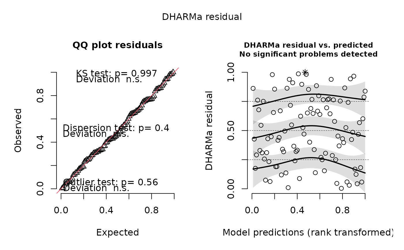
# the plot function shows 2 plots and runs 4 tests
# i) KS test i) Dispersion test iii) Outlier test iv) quantile test
plot(simulationOutput, quantreg = TRUE)
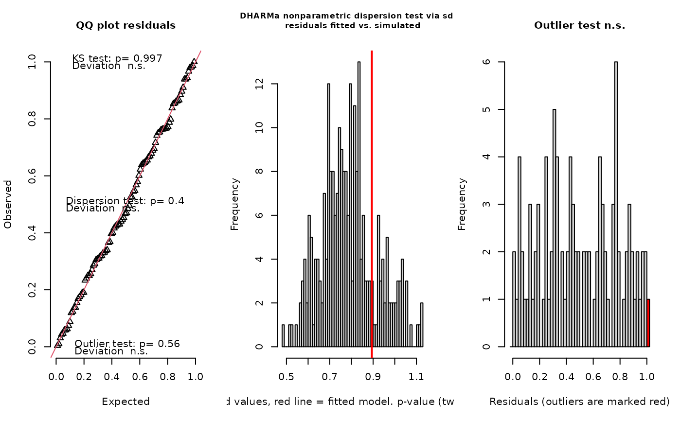
 # testResiduals tests distribution, dispersion and outliers
testResiduals(simulationOutput)
# testResiduals tests distribution, dispersion and outliers
testResiduals(simulationOutput)
 #> $uniformity
#>
#> Asymptotic one-sample Kolmogorov-Smirnov test
#>
#> data: simulationOutput$scaledResiduals
#> D = 0.040188, p-value = 0.997
#> alternative hypothesis: two-sided
#>
#>
#> $dispersion
#>
#> DHARMa nonparametric dispersion test via sd of residuals fitted vs.
#> simulated
#>
#> data: simulationOutput
#> dispersion = 1.1341, p-value = 0.4
#> alternative hypothesis: two.sided
#>
#>
#> $outliers
#>
#> DHARMa bootstrapped outlier test
#>
#> data: simulationOutput
#> outliers at both margin(s) = 1, observations = 100, p-value = 0.6
#> alternative hypothesis: two.sided
#> percent confidence interval:
#> 0.00 0.02
#> sample estimates:
#> outlier frequency (expected: 0.0036 )
#> 0.01
#>
#>
####### Individual tests #######
# KS test for correct distribution of residuals
testUniformity(simulationOutput)
#> $uniformity
#>
#> Asymptotic one-sample Kolmogorov-Smirnov test
#>
#> data: simulationOutput$scaledResiduals
#> D = 0.040188, p-value = 0.997
#> alternative hypothesis: two-sided
#>
#>
#> $dispersion
#>
#> DHARMa nonparametric dispersion test via sd of residuals fitted vs.
#> simulated
#>
#> data: simulationOutput
#> dispersion = 1.1341, p-value = 0.4
#> alternative hypothesis: two.sided
#>
#>
#> $outliers
#>
#> DHARMa bootstrapped outlier test
#>
#> data: simulationOutput
#> outliers at both margin(s) = 1, observations = 100, p-value = 0.6
#> alternative hypothesis: two.sided
#> percent confidence interval:
#> 0.00 0.02
#> sample estimates:
#> outlier frequency (expected: 0.0036 )
#> 0.01
#>
#>
####### Individual tests #######
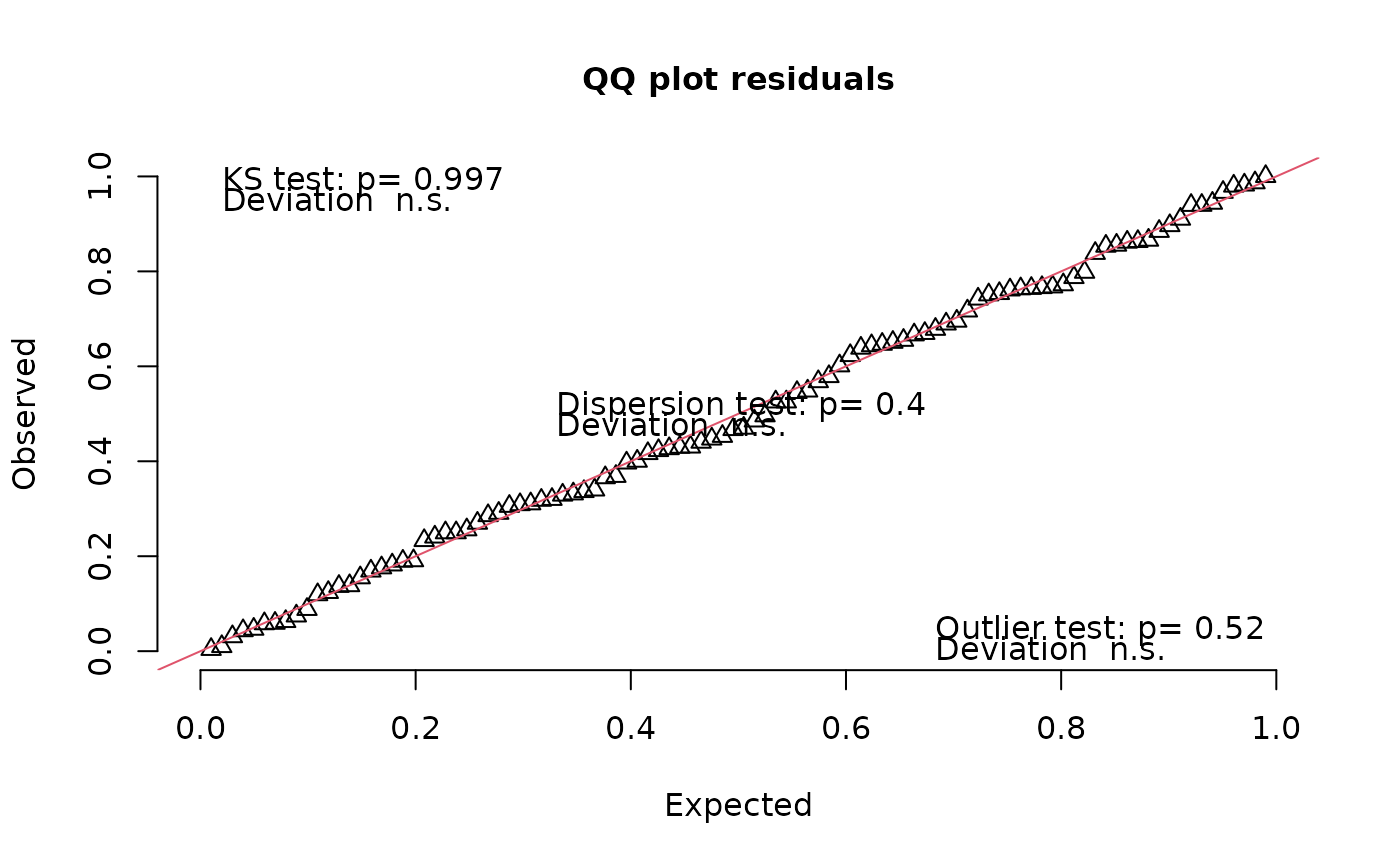
# KS test for correct distribution of residuals
testUniformity(simulationOutput)
 #>
#> Asymptotic one-sample Kolmogorov-Smirnov test
#>
#> data: simulationOutput$scaledResiduals
#> D = 0.040188, p-value = 0.997
#> alternative hypothesis: two-sided
#>
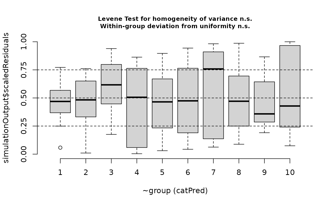
# KS test for correct distribution within and between groups
# group specified as formula (recommended)
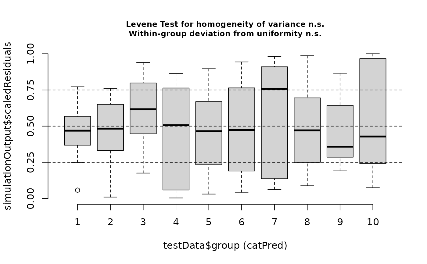
testCategorical(simulationOutput, ~group)
#>
#> Asymptotic one-sample Kolmogorov-Smirnov test
#>
#> data: simulationOutput$scaledResiduals
#> D = 0.040188, p-value = 0.997
#> alternative hypothesis: two-sided
#>
# KS test for correct distribution within and between groups
# group specified as formula (recommended)
testCategorical(simulationOutput, ~group)
 #> $uniformity
$details
#> catPred: 1
#>
#> Exact one-sample Kolmogorov-Smirnov test
#>
#> data: dd[x, ]
#> D = 0.23215, p-value = 0.5771
#> alternative hypothesis: two-sided
#>
#> ------------------------------------------------------------
#> catPred: 2
#>
#> Exact one-sample Kolmogorov-Smirnov test
#>
#> data: dd[x, ]
#> D = 0.23894, p-value = 0.541
#> alternative hypothesis: two-sided
#>
#> ------------------------------------------------------------
#> catPred: 3
#>
#> Exact one-sample Kolmogorov-Smirnov test
#>
#> data: dd[x, ]
#> D = 0.32967, p-value = 0.1809
#> alternative hypothesis: two-sided
#>
#> ------------------------------------------------------------
#> catPred: 4
#>
#> Exact one-sample Kolmogorov-Smirnov test
#>
#> data: dd[x, ]
#> D = 0.24106, p-value = 0.5299
#> alternative hypothesis: two-sided
#>
#> ------------------------------------------------------------
#> catPred: 5
#>
#> Exact one-sample Kolmogorov-Smirnov test
#>
#> data: dd[x, ]
#> D = 0.18324, p-value = 0.8322
#> alternative hypothesis: two-sided
#>
#> ------------------------------------------------------------
#> catPred: 6
#>
#> Exact one-sample Kolmogorov-Smirnov test
#>
#> data: dd[x, ]
#> D = 0.15352, p-value = 0.9449
#> alternative hypothesis: two-sided
#>
#> ------------------------------------------------------------
#> catPred: 7
#>
#> Exact one-sample Kolmogorov-Smirnov test
#>
#> data: dd[x, ]
#> D = 0.33805, p-value = 0.1602
#> alternative hypothesis: two-sided
#>
#> ------------------------------------------------------------
#> catPred: 8
#>
#> Exact one-sample Kolmogorov-Smirnov test
#>
#> data: dd[x, ]
#> D = 0.15491, p-value = 0.9411
#> alternative hypothesis: two-sided
#>
#> ------------------------------------------------------------
#> catPred: 9
#>
#> Exact one-sample Kolmogorov-Smirnov test
#>
#> data: dd[x, ]
#> D = 0.27727, p-value = 0.3576
#> alternative hypothesis: two-sided
#>
#> ------------------------------------------------------------
#> catPred: 10
#>
#> Exact one-sample Kolmogorov-Smirnov test
#>
#> data: dd[x, ]
#> D = 0.26664, p-value = 0.4042
#> alternative hypothesis: two-sided
#>
#>
#> $uniformity$p.value
#> [1] 0.5770857 0.5410355 0.1809108 0.5299309 0.8322467 0.9449449 0.1602026
#> [8] 0.9411058 0.3575947 0.4042000
#>
#> $uniformity$p.value.cor
#> [1] 1 1 1 1 1 1 1 1 1 1
#>
#>
#> $homogeneity
#> Levene's Test for Homogeneity of Variance (center = median)
#> Df F value Pr(>F)
#> group 9 1.2646 0.2672
#> 90
#>
# group specified as variable in your environment
testCategorical(simulationOutput, testData$group)
#> $uniformity
#> $uniformity$details
#> catPred: 1
#>
#> Exact one-sample Kolmogorov-Smirnov test
#>
#> data: dd[x, ]
#> D = 0.23215, p-value = 0.5771
#> alternative hypothesis: two-sided
#>
#> ------------------------------------------------------------
#> catPred: 2
#>
#> Exact one-sample Kolmogorov-Smirnov test
#>
#> data: dd[x, ]
#> D = 0.23894, p-value = 0.541
#> alternative hypothesis: two-sided
#>
#> ------------------------------------------------------------
#> catPred: 3
#>
#> Exact one-sample Kolmogorov-Smirnov test
#>
#> data: dd[x, ]
#> D = 0.32967, p-value = 0.1809
#> alternative hypothesis: two-sided
#>
#> ------------------------------------------------------------
#> catPred: 4
#>
#> Exact one-sample Kolmogorov-Smirnov test
#>
#> data: dd[x, ]
#> D = 0.24106, p-value = 0.5299
#> alternative hypothesis: two-sided
#>
#> ------------------------------------------------------------
#> catPred: 5
#>
#> Exact one-sample Kolmogorov-Smirnov test
#>
#> data: dd[x, ]
#> D = 0.18324, p-value = 0.8322
#> alternative hypothesis: two-sided
#>
#> ------------------------------------------------------------
#> catPred: 6
#>
#> Exact one-sample Kolmogorov-Smirnov test
#>
#> data: dd[x, ]
#> D = 0.15352, p-value = 0.9449
#> alternative hypothesis: two-sided
#>
#> ------------------------------------------------------------
#> catPred: 7
#>
#> Exact one-sample Kolmogorov-Smirnov test
#>
#> data: dd[x, ]
#> D = 0.33805, p-value = 0.1602
#> alternative hypothesis: two-sided
#>
#> ------------------------------------------------------------
#> catPred: 8
#>
#> Exact one-sample Kolmogorov-Smirnov test
#>
#> data: dd[x, ]
#> D = 0.15491, p-value = 0.9411
#> alternative hypothesis: two-sided
#>
#> ------------------------------------------------------------
#> catPred: 9
#>
#> Exact one-sample Kolmogorov-Smirnov test
#>
#> data: dd[x, ]
#> D = 0.27727, p-value = 0.3576
#> alternative hypothesis: two-sided
#>
#> ------------------------------------------------------------
#> catPred: 10
#>
#> Exact one-sample Kolmogorov-Smirnov test
#>
#> data: dd[x, ]
#> D = 0.26664, p-value = 0.4042
#> alternative hypothesis: two-sided
#>
#>
#> $uniformity$p.value
#> [1] 0.5770857 0.5410355 0.1809108 0.5299309 0.8322467 0.9449449 0.1602026
#> [8] 0.9411058 0.3575947 0.4042000
#>
#> $uniformity$p.value.cor
#> [1] 1 1 1 1 1 1 1 1 1 1
#>
#>
#> $homogeneity
#> Levene's Test for Homogeneity of Variance (center = median)
#> Df F value Pr(>F)
#> group 9 1.2646 0.2672
#> 90
#>
# group specified as variable in your environment
testCategorical(simulationOutput, testData$group)
 #> $uniformity
$details
#> catPred: 1
#>
#> Exact one-sample Kolmogorov-Smirnov test
#>
#> data: dd[x, ]
#> D = 0.23215, p-value = 0.5771
#> alternative hypothesis: two-sided
#>
#> ------------------------------------------------------------
#> catPred: 2
#>
#> Exact one-sample Kolmogorov-Smirnov test
#>
#> data: dd[x, ]
#> D = 0.23894, p-value = 0.541
#> alternative hypothesis: two-sided
#>
#> ------------------------------------------------------------
#> catPred: 3
#>
#> Exact one-sample Kolmogorov-Smirnov test
#>
#> data: dd[x, ]
#> D = 0.32967, p-value = 0.1809
#> alternative hypothesis: two-sided
#>
#> ------------------------------------------------------------
#> catPred: 4
#>
#> Exact one-sample Kolmogorov-Smirnov test
#>
#> data: dd[x, ]
#> D = 0.24106, p-value = 0.5299
#> alternative hypothesis: two-sided
#>
#> ------------------------------------------------------------
#> catPred: 5
#>
#> Exact one-sample Kolmogorov-Smirnov test
#>
#> data: dd[x, ]
#> D = 0.18324, p-value = 0.8322
#> alternative hypothesis: two-sided
#>
#> ------------------------------------------------------------
#> catPred: 6
#>
#> Exact one-sample Kolmogorov-Smirnov test
#>
#> data: dd[x, ]
#> D = 0.15352, p-value = 0.9449
#> alternative hypothesis: two-sided
#>
#> ------------------------------------------------------------
#> catPred: 7
#>
#> Exact one-sample Kolmogorov-Smirnov test
#>
#> data: dd[x, ]
#> D = 0.33805, p-value = 0.1602
#> alternative hypothesis: two-sided
#>
#> ------------------------------------------------------------
#> catPred: 8
#>
#> Exact one-sample Kolmogorov-Smirnov test
#>
#> data: dd[x, ]
#> D = 0.15491, p-value = 0.9411
#> alternative hypothesis: two-sided
#>
#> ------------------------------------------------------------
#> catPred: 9
#>
#> Exact one-sample Kolmogorov-Smirnov test
#>
#> data: dd[x, ]
#> D = 0.27727, p-value = 0.3576
#> alternative hypothesis: two-sided
#>
#> ------------------------------------------------------------
#> catPred: 10
#>
#> Exact one-sample Kolmogorov-Smirnov test
#>
#> data: dd[x, ]
#> D = 0.26664, p-value = 0.4042
#> alternative hypothesis: two-sided
#>
#>
#> $uniformity$p.value
#> [1] 0.5770857 0.5410355 0.1809108 0.5299309 0.8322467 0.9449449 0.1602026
#> [8] 0.9411058 0.3575947 0.4042000
#>
#> $uniformity$p.value.cor
#> [1] 1 1 1 1 1 1 1 1 1 1
#>
#>
#> $homogeneity
#> Levene's Test for Homogeneity of Variance (center = median)
#> Df F value Pr(>F)
#> group 9 1.2646 0.2672
#> 90
#>
# Dispersion test - for details see ?testDispersion
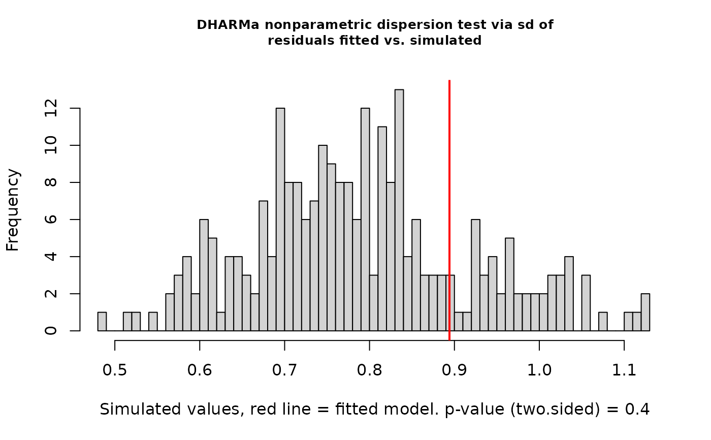
testDispersion(simulationOutput) # tests under and overdispersion
#> $uniformity
#> $uniformity$details
#> catPred: 1
#>
#> Exact one-sample Kolmogorov-Smirnov test
#>
#> data: dd[x, ]
#> D = 0.23215, p-value = 0.5771
#> alternative hypothesis: two-sided
#>
#> ------------------------------------------------------------
#> catPred: 2
#>
#> Exact one-sample Kolmogorov-Smirnov test
#>
#> data: dd[x, ]
#> D = 0.23894, p-value = 0.541
#> alternative hypothesis: two-sided
#>
#> ------------------------------------------------------------
#> catPred: 3
#>
#> Exact one-sample Kolmogorov-Smirnov test
#>
#> data: dd[x, ]
#> D = 0.32967, p-value = 0.1809
#> alternative hypothesis: two-sided
#>
#> ------------------------------------------------------------
#> catPred: 4
#>
#> Exact one-sample Kolmogorov-Smirnov test
#>
#> data: dd[x, ]
#> D = 0.24106, p-value = 0.5299
#> alternative hypothesis: two-sided
#>
#> ------------------------------------------------------------
#> catPred: 5
#>
#> Exact one-sample Kolmogorov-Smirnov test
#>
#> data: dd[x, ]
#> D = 0.18324, p-value = 0.8322
#> alternative hypothesis: two-sided
#>
#> ------------------------------------------------------------
#> catPred: 6
#>
#> Exact one-sample Kolmogorov-Smirnov test
#>
#> data: dd[x, ]
#> D = 0.15352, p-value = 0.9449
#> alternative hypothesis: two-sided
#>
#> ------------------------------------------------------------
#> catPred: 7
#>
#> Exact one-sample Kolmogorov-Smirnov test
#>
#> data: dd[x, ]
#> D = 0.33805, p-value = 0.1602
#> alternative hypothesis: two-sided
#>
#> ------------------------------------------------------------
#> catPred: 8
#>
#> Exact one-sample Kolmogorov-Smirnov test
#>
#> data: dd[x, ]
#> D = 0.15491, p-value = 0.9411
#> alternative hypothesis: two-sided
#>
#> ------------------------------------------------------------
#> catPred: 9
#>
#> Exact one-sample Kolmogorov-Smirnov test
#>
#> data: dd[x, ]
#> D = 0.27727, p-value = 0.3576
#> alternative hypothesis: two-sided
#>
#> ------------------------------------------------------------
#> catPred: 10
#>
#> Exact one-sample Kolmogorov-Smirnov test
#>
#> data: dd[x, ]
#> D = 0.26664, p-value = 0.4042
#> alternative hypothesis: two-sided
#>
#>
#> $uniformity$p.value
#> [1] 0.5770857 0.5410355 0.1809108 0.5299309 0.8322467 0.9449449 0.1602026
#> [8] 0.9411058 0.3575947 0.4042000
#>
#> $uniformity$p.value.cor
#> [1] 1 1 1 1 1 1 1 1 1 1
#>
#>
#> $homogeneity
#> Levene's Test for Homogeneity of Variance (center = median)
#> Df F value Pr(>F)
#> group 9 1.2646 0.2672
#> 90
#>
# Dispersion test - for details see ?testDispersion
testDispersion(simulationOutput) # tests under and overdispersion
 #>
#> DHARMa nonparametric dispersion test via sd of residuals fitted vs.
#> simulated
#>
#> data: simulationOutput
#> dispersion = 1.1341, p-value = 0.4
#> alternative hypothesis: two.sided
#>
# Outlier test (number of observations outside simulation envelope)
# Use type = "boostrap" for exact values, see ?testOutliers
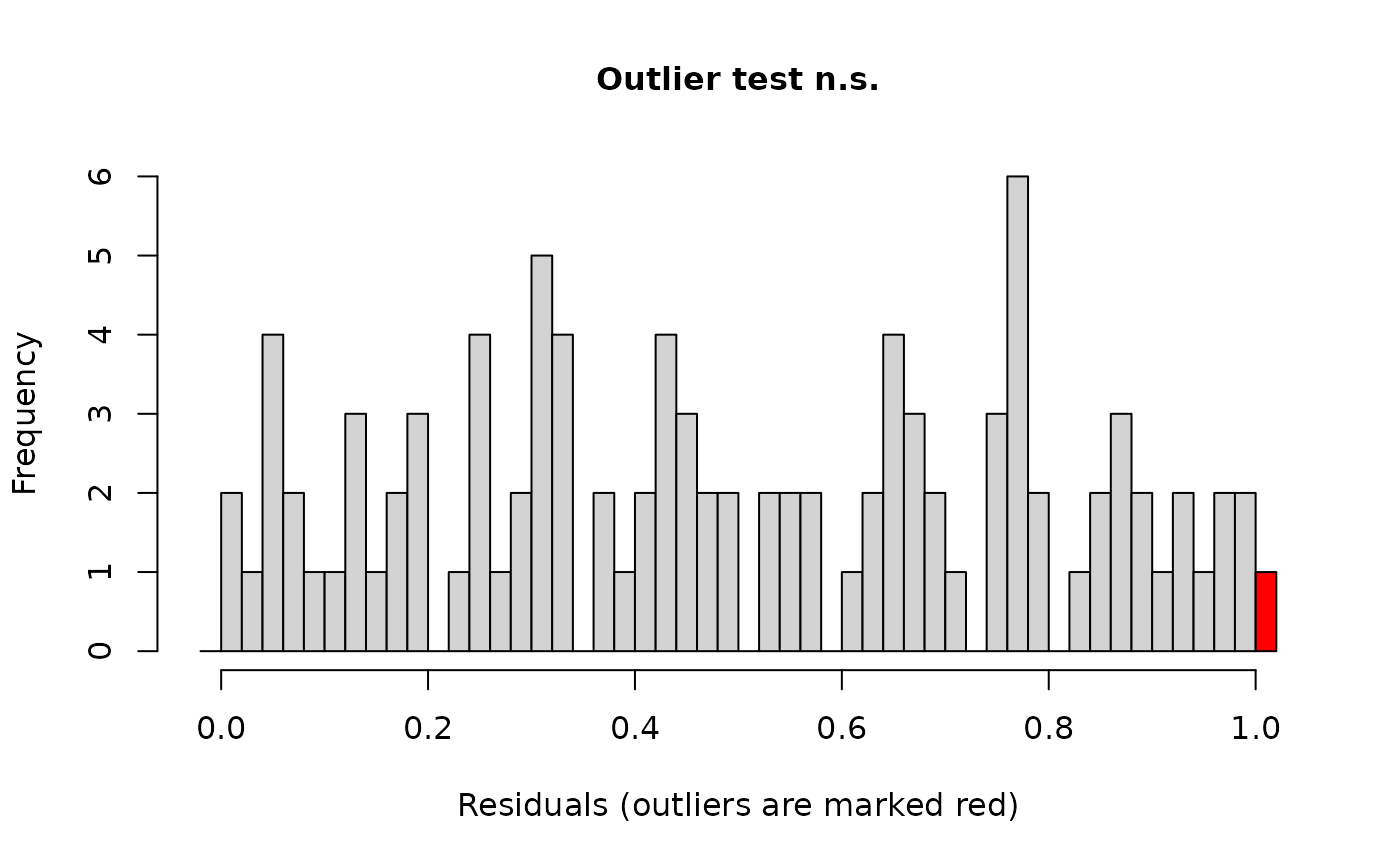
testOutliers(simulationOutput, type = "binomial")
#>
#> DHARMa nonparametric dispersion test via sd of residuals fitted vs.
#> simulated
#>
#> data: simulationOutput
#> dispersion = 1.1341, p-value = 0.4
#> alternative hypothesis: two.sided
#>
# Outlier test (number of observations outside simulation envelope)
# Use type = "boostrap" for exact values, see ?testOutliers
testOutliers(simulationOutput, type = "binomial")
 #>
#> DHARMa outlier test based on exact binomial test with approximate
#> expectations
#>
#> data: simulationOutput
#> outliers at both margin(s) = 2, observations = 100, p-value = 0.1898
#> alternative hypothesis: true probability of success is not equal to 0.007968127
#> 95 percent confidence interval:
#> 0.002431337 0.070383932
#> sample estimates:
#> frequency of outliers (expected: 0.00796812749003984 )
#> 0.02
#>
# testing zero inflation
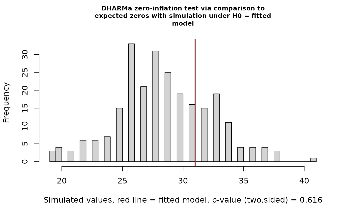
testZeroInflation(simulationOutput)
#>
#> DHARMa outlier test based on exact binomial test with approximate
#> expectations
#>
#> data: simulationOutput
#> outliers at both margin(s) = 2, observations = 100, p-value = 0.1898
#> alternative hypothesis: true probability of success is not equal to 0.007968127
#> 95 percent confidence interval:
#> 0.002431337 0.070383932
#> sample estimates:
#> frequency of outliers (expected: 0.00796812749003984 )
#> 0.02
#>
# testing zero inflation
testZeroInflation(simulationOutput)
 #>
#> DHARMa zero-inflation test via comparison to expected zeros with
#> simulation under H0 = fitted model
#>
#> data: simulationOutput
#> ratioObsSim = 1.0816, p-value = 0.616
#> alternative hypothesis: two.sided
#>
# testing generic summaries
countOnes <- function(x) sum(x == 1) # testing for number of 1s
testGeneric(simulationOutput, summary = countOnes) # 1-inflation
#>
#> DHARMa zero-inflation test via comparison to expected zeros with
#> simulation under H0 = fitted model
#>
#> data: simulationOutput
#> ratioObsSim = 1.0816, p-value = 0.616
#> alternative hypothesis: two.sided
#>
# testing generic summaries
countOnes <- function(x) sum(x == 1) # testing for number of 1s
testGeneric(simulationOutput, summary = countOnes) # 1-inflation
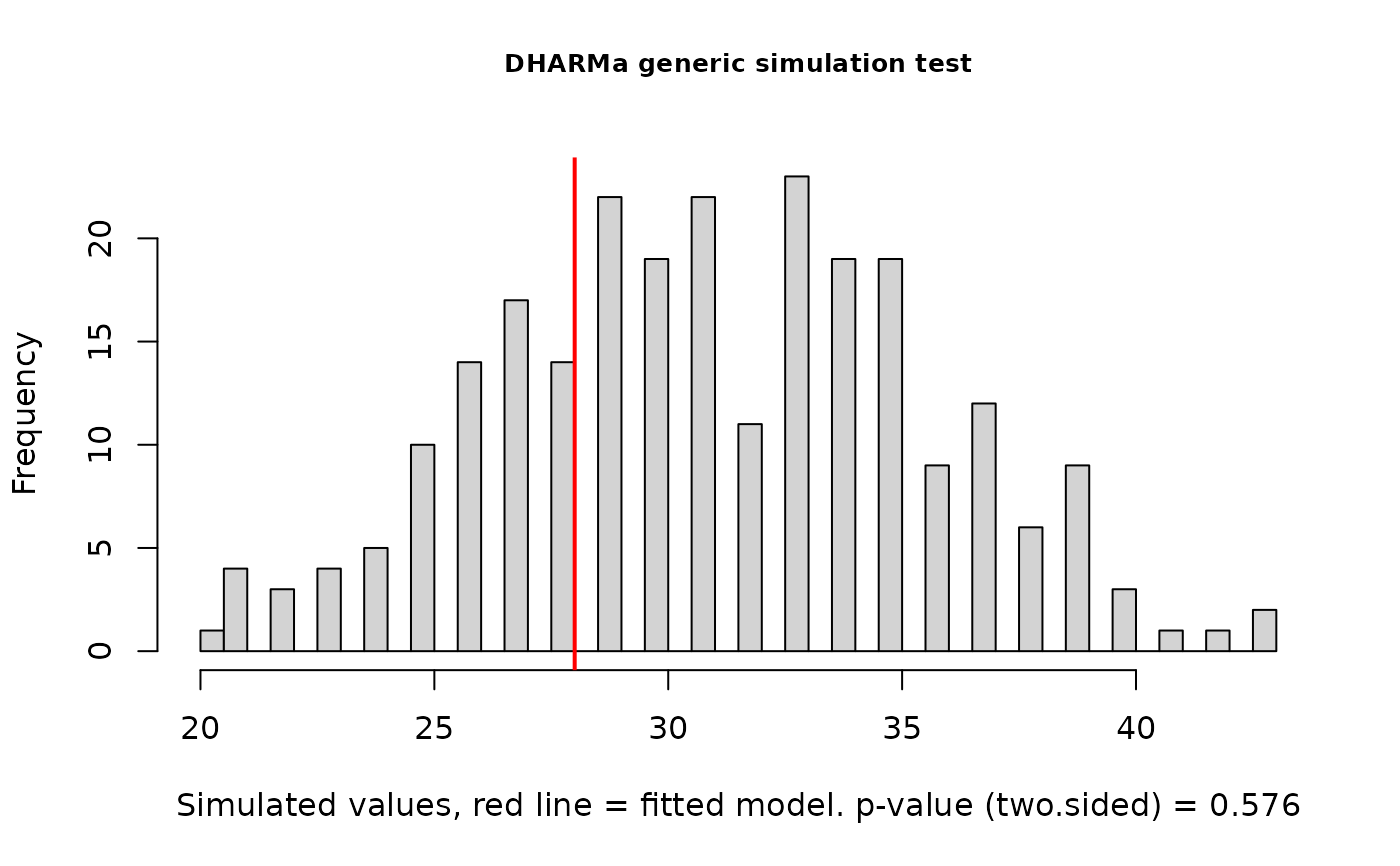 #>
#> DHARMa generic simulation test
#>
#> data: simulationOutput
#> ratioObsSim = 0.89801, p-value = 0.576
#> alternative hypothesis: two.sided
#>
testGeneric(simulationOutput, summary = countOnes, alternative = "less") # 1-deficit
#>
#> DHARMa generic simulation test
#>
#> data: simulationOutput
#> ratioObsSim = 0.89801, p-value = 0.576
#> alternative hypothesis: two.sided
#>
testGeneric(simulationOutput, summary = countOnes, alternative = "less") # 1-deficit
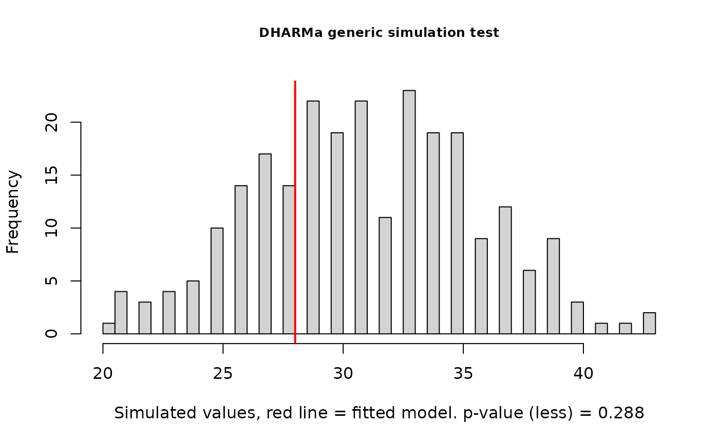 #>
#> DHARMa generic simulation test
#>
#> data: simulationOutput
#> ratioObsSim = 0.89801, p-value = 0.288
#> alternative hypothesis: less
#>
means <- function(x) mean(x) # testing if mean prediction fits
testGeneric(simulationOutput, summary = means)
#>
#> DHARMa generic simulation test
#>
#> data: simulationOutput
#> ratioObsSim = 0.89801, p-value = 0.288
#> alternative hypothesis: less
#>
means <- function(x) mean(x) # testing if mean prediction fits
testGeneric(simulationOutput, summary = means)
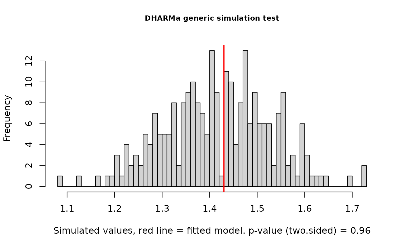 #>
#> DHARMa generic simulation test
#>
#> data: simulationOutput
#> ratioObsSim = 1.006, p-value = 0.96
#> alternative hypothesis: two.sided
#>
spread <- function(x) sd(x) # testing if mean sd fits
testGeneric(simulationOutput, summary = spread)
#>
#> DHARMa generic simulation test
#>
#> data: simulationOutput
#> ratioObsSim = 1.006, p-value = 0.96
#> alternative hypothesis: two.sided
#>
spread <- function(x) sd(x) # testing if mean sd fits
testGeneric(simulationOutput, summary = spread)
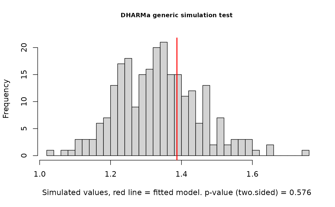 #>
#> DHARMa generic simulation test
#>
#> data: simulationOutput
#> ratioObsSim = 1.0387, p-value = 0.576
#> alternative hypothesis: two.sided
#>
#>
#> DHARMa generic simulation test
#>
#> data: simulationOutput
#> ratioObsSim = 1.0387, p-value = 0.576
#> alternative hypothesis: two.sided
#>