The purpose of this function is to recalculate scaled residuals per group, based on the simulations done by simulateResiduals.
Usage
recalculateResiduals(simulationOutput, group = NULL, aggregateBy = sum,
  sel = NULL, seed = 123, method = c("PIT", "traditional"),
  rotation = NULL)
Arguments
- simulationOutput
an object with simulated residuals created by simulateResiduals.
- group
a grouping variable with the same dimensions as the residuals in simulationOutput. If specified as formula, e.g. group = ~group, NAs are handled automatically (recommended).
- aggregateBy
function for the aggregation. Default is sum. This should only be changed if you know what you are doing. Note in particular that the expected residual distribution might not be flat anymore if you choose general functions, such as sd etc.
- sel
an optional vector for selecting the data to be aggregated.
- seed
the random seed to be used within DHARMa. The default setting, recommended for most users, is to keep the random seed on a fixed value of 123. This means that you will always get the same randomization and thus the same result when running the same code. NULL = no new seed is set, but previous random state will be restored after simulation. FALSE = no seed is set, and random state will not be restored. The latter two options are only recommended for simulation experiments. See vignette for details.
- method
the quantile randomization method used. The two options implemented at the moment are probability integral transform (PIT-) residuals (current default), and the "traditional" randomization procedure, that was used in DHARMa until version 0.3.0. For details, see getQuantile.
- rotation
optional rotation of the residual space to remove residual autocorrelation. See details in simulateResiduals, section residual auto-correlation for an extended explanation, and getQuantile for syntax.
Value
an object of class DHARMa, similar to what is returned by simulateResiduals, but with additional outputs for the new grouped calculations. Note that the relevant outputs are 2x in the object, the first is the grouped calculations (which is returned by $name access), and later another time, under identical name, the original output. Moreover, there is a function 'aggregateByGroup', which can be used to aggregate predictor variables in the same way as the variables calculated here.
Details
The function aggregates the observed and simulated data per group according to the function provided by the aggregateBy option. DHARMa residuals are then calculated exactly as for a single data point (see getQuantile for details).
Examples
library(lme4)
#> Loading required package: Matrix
#>
#> Attaching package: ‘lme4’
#> The following object is masked from ‘package:DHARMa’:
#>
#> getData
testData = createData(sampleSize = 100, overdispersion = 0.5, family = poisson())
fittedModel <- glmer(observedResponse ~ Environment1 + (1|group),
family = "poisson", data = testData)
# simulate residuals (default behavior, conditional on the fitted random effects)
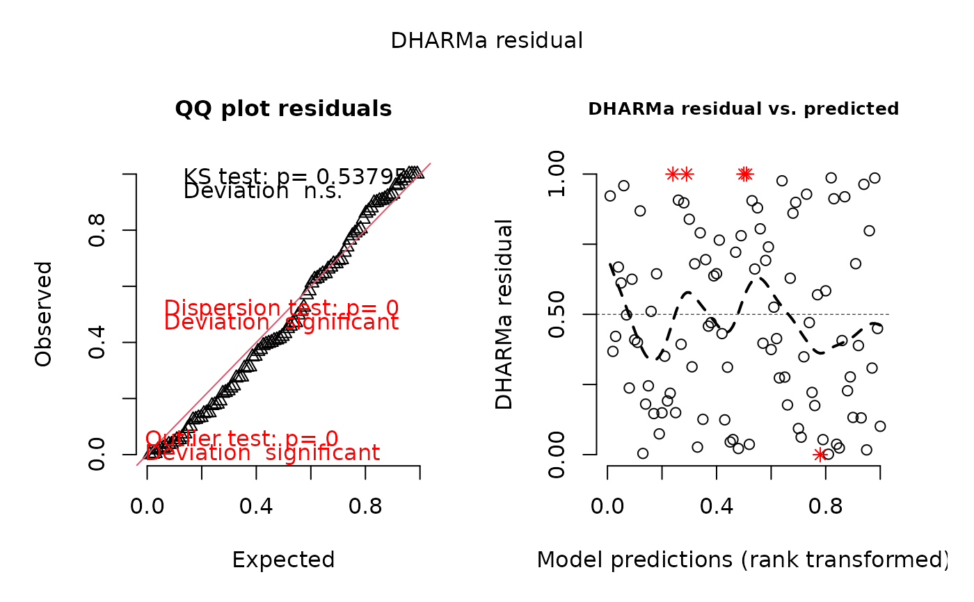
simulationOutput1 <- simulateResiduals(fittedModel = fittedModel)
plot(simulationOutput1, quantreg = FALSE)
 # simulate residuals unconditional on the fitted random effects (REs are re-simulated)
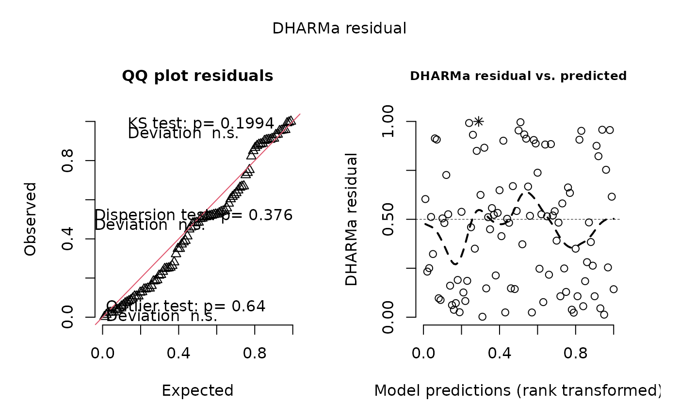
simulationOutput2 <- simulateResiduals(fittedModel = fittedModel,
simulateREs = "unconditional")
plot(simulationOutput2, quantreg = FALSE)
# simulate residuals unconditional on the fitted random effects (REs are re-simulated)
simulationOutput2 <- simulateResiduals(fittedModel = fittedModel,
simulateREs = "unconditional")
plot(simulationOutput2, quantreg = FALSE)
 # simulate residuals user-specified using lme4 syntax (e.g. conditional only on a specific RE)
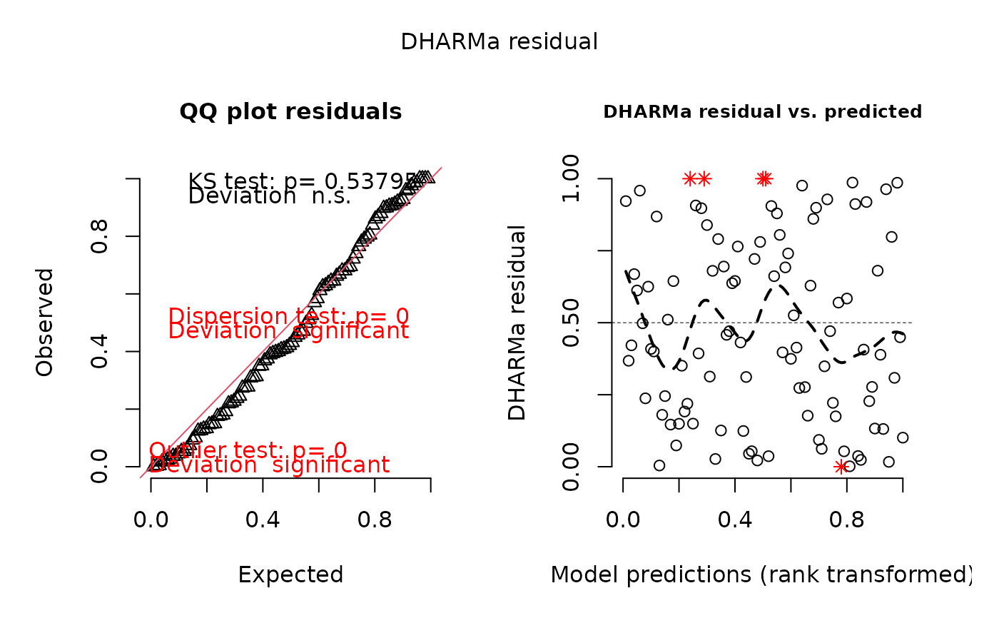
simulationOutput3 <- simulateResiduals(fittedModel = fittedModel,
simulateREs = "user-specified",
re.form = ~(1|group))
plot(simulationOutput3, quantreg = FALSE)
# simulate residuals user-specified using lme4 syntax (e.g. conditional only on a specific RE)
simulationOutput3 <- simulateResiduals(fittedModel = fittedModel,
simulateREs = "user-specified",
re.form = ~(1|group))
plot(simulationOutput3, quantreg = FALSE)
 # one of the possible test, for other options see ?testResiduals / vignette
testDispersion(simulationOutput1)
# one of the possible test, for other options see ?testResiduals / vignette
testDispersion(simulationOutput1)
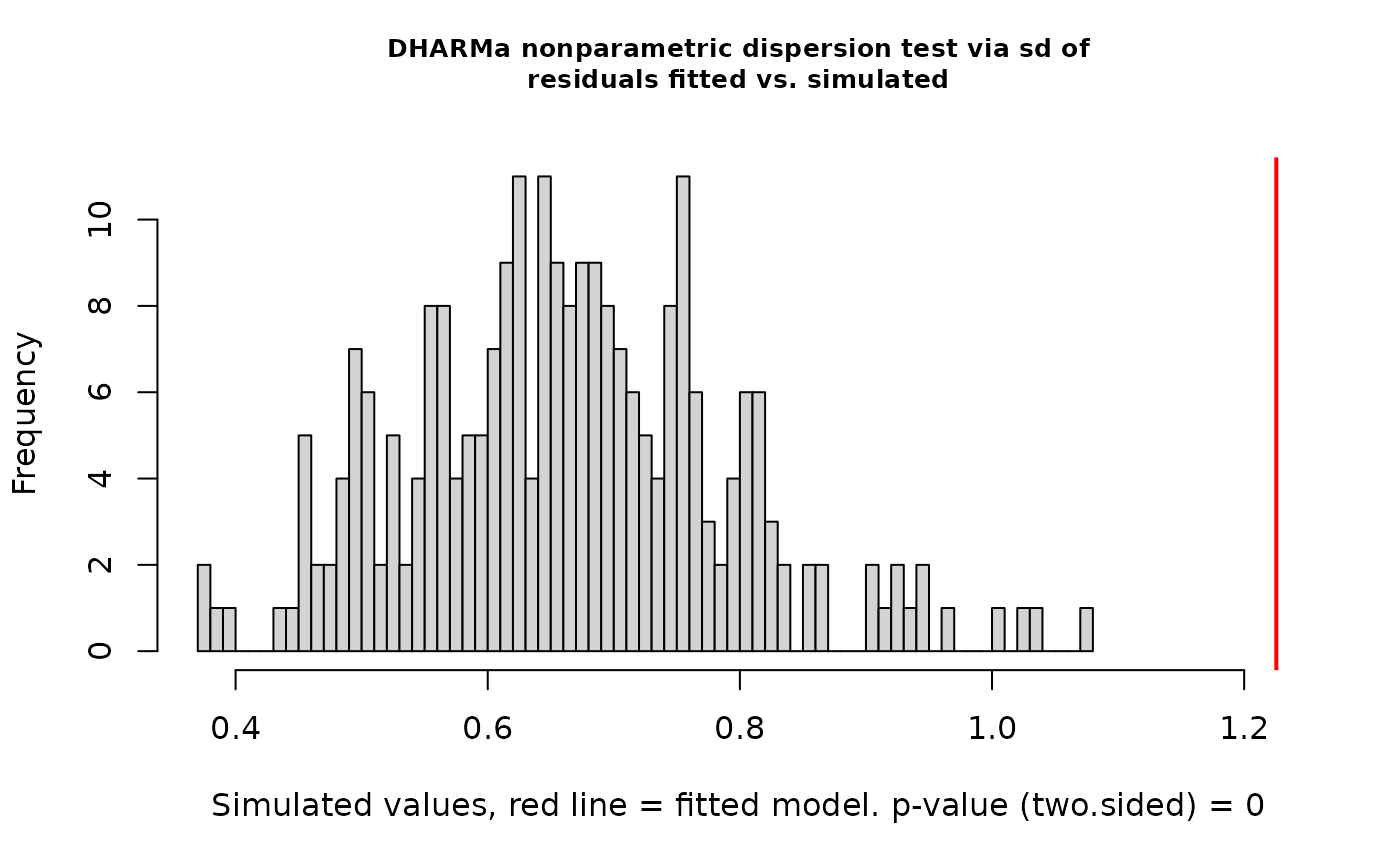 #>
#> DHARMa nonparametric dispersion test via sd of residuals fitted vs.
#> simulated
#>
#> data: simulationOutput
#> dispersion = 1.847, p-value < 2.2e-16
#> alternative hypothesis: two.sided
#>
# the calculated residuals can be accessed via
residuals(simulationOutput1)
#> [1] 0.036590673 0.174908432 0.680523482 0.740300219 0.180170371 0.125794095
#> [7] 0.001503811 0.963353192 0.985899959 0.149059348 0.628721685 0.911976527
#> [13] 0.409114103 0.497978346 0.431352814 0.045102526 0.073961475 0.149618790
#> [19] 1.000000000 0.026836112 0.457930113 0.721381689 0.899130944 0.525581610
#> [25] 0.879506408 0.123994000 0.611803926 0.393362344 0.016866707 0.668601542
#> [31] 0.839019117 0.100964543 0.276995893 1.000000000 0.625202295 0.308584325
#> [37] 0.177185447 0.237491989 0.406646840 0.421516509 0.350742962 0.348665736
#> [43] 0.132608657 0.583864983 0.131003213 0.922074926 0.958540510 0.637011220
#> [49] 0.191546867 0.868639081 1.000000000 0.367920206 0.245235073 0.797861902
#> [55] 0.021743049 0.569822114 0.975968427 0.023692987 0.449477576 0.413590558
#> [61] 0.037088446 0.780333111 0.470484520 0.510608368 0.146277531 0.790458441
#> [67] 0.764489104 0.804808478 0.053457780 0.928182991 0.221726895 0.053761322
#> [73] 0.919086938 0.644490416 0.470611219 0.312944008 0.860487860 0.273356538
#> [79] 0.004266388 0.397041753 0.644881394 0.400107773 0.986513846 0.276370811
#> [85] 0.695016811 0.897446885 0.218763697 0.227667090 0.311519663 0.093117996
#> [91] 0.661566506 0.062156748 0.388783699 0.374589793 1.000000000 0.680056192
#> [97] 0.000000000 0.905033439 0.906951471 0.692050004
# transform residuals to other pdf, see ?residuals.DHARMa for details
residuals(simulationOutput1, quantileFunction = qnorm, outlierValues = c(-7,7))
#> [1] -1.791698058 -0.934944575 0.469163132 0.644271240 -0.914716000
#> [6] -1.146500332 -2.966957768 1.790998000 2.194491668 -1.040476243
#> [11] 0.328469595 1.353027184 -0.229824422 -0.005067556 -0.172931047
#> [16] -1.694317057 -1.446907080 -1.038069759 7.000000000 -1.929472552
#> [21] -0.105649782 0.586950992 1.276615257 0.064167594 1.172522901
#> [26] -1.155250159 0.284023793 -0.270566210 -2.123243958 0.436054874
#> [31] 0.990434546 -1.276074777 -0.591789155 7.000000000 0.319172893
#> [36] -0.499867112 -0.926144494 -0.714393359 -0.236179121 -0.198015396
#> [41] -0.383315397 -0.388925210 -1.114144237 0.211791071 -1.121661422
#> [46] 1.419167636 1.733994947 0.350481250 -0.872210168 1.119981047
#> [51] 7.000000000 -0.337366796 -0.689561244 0.834008496 -2.019010792
#> [56] 0.175921299 1.976809697 -1.982834009 -0.126981359 -0.218318302
#> [61] -1.785520730 0.773318722 -0.074051960 0.026594370 -1.052533037
#> [66] 0.808012967 0.720817525 0.858922918 -1.612213173 1.462391280
#> [71] -0.766374013 -1.609428653 1.398956180 0.370487661 -0.073733506
#> [76] -0.487522621 1.082513814 -0.602692794 -2.630227450 -0.261011673
#> [81] 0.371537525 -0.253068156 2.211918331 -0.593656891 0.510121451
#> [86] 1.267137215 -0.776375350 -0.746551754 -0.491547414 -1.321796296
#> [91] 0.416742194 -1.536917572 -0.282490542 -0.319721335 7.000000000
#> [96] 0.467855937 -7.000000000 1.310776983 1.322213527 0.501669543
# get residuals that are outside the simulation envelope
outliers(simulationOutput1)
#> [1] 19 34 51 95 97
# calculating aggregated residuals per group
# group here specified as formula (recommended)
# but you can also use a variable from your environment, e.g. testData$group
simulationOutput4 = recalculateResiduals(simulationOutput1, group = ~group)
plot(simulationOutput4, quantreg = FALSE)
#>
#> DHARMa nonparametric dispersion test via sd of residuals fitted vs.
#> simulated
#>
#> data: simulationOutput
#> dispersion = 1.847, p-value < 2.2e-16
#> alternative hypothesis: two.sided
#>
# the calculated residuals can be accessed via
residuals(simulationOutput1)
#> [1] 0.036590673 0.174908432 0.680523482 0.740300219 0.180170371 0.125794095
#> [7] 0.001503811 0.963353192 0.985899959 0.149059348 0.628721685 0.911976527
#> [13] 0.409114103 0.497978346 0.431352814 0.045102526 0.073961475 0.149618790
#> [19] 1.000000000 0.026836112 0.457930113 0.721381689 0.899130944 0.525581610
#> [25] 0.879506408 0.123994000 0.611803926 0.393362344 0.016866707 0.668601542
#> [31] 0.839019117 0.100964543 0.276995893 1.000000000 0.625202295 0.308584325
#> [37] 0.177185447 0.237491989 0.406646840 0.421516509 0.350742962 0.348665736
#> [43] 0.132608657 0.583864983 0.131003213 0.922074926 0.958540510 0.637011220
#> [49] 0.191546867 0.868639081 1.000000000 0.367920206 0.245235073 0.797861902
#> [55] 0.021743049 0.569822114 0.975968427 0.023692987 0.449477576 0.413590558
#> [61] 0.037088446 0.780333111 0.470484520 0.510608368 0.146277531 0.790458441
#> [67] 0.764489104 0.804808478 0.053457780 0.928182991 0.221726895 0.053761322
#> [73] 0.919086938 0.644490416 0.470611219 0.312944008 0.860487860 0.273356538
#> [79] 0.004266388 0.397041753 0.644881394 0.400107773 0.986513846 0.276370811
#> [85] 0.695016811 0.897446885 0.218763697 0.227667090 0.311519663 0.093117996
#> [91] 0.661566506 0.062156748 0.388783699 0.374589793 1.000000000 0.680056192
#> [97] 0.000000000 0.905033439 0.906951471 0.692050004
# transform residuals to other pdf, see ?residuals.DHARMa for details
residuals(simulationOutput1, quantileFunction = qnorm, outlierValues = c(-7,7))
#> [1] -1.791698058 -0.934944575 0.469163132 0.644271240 -0.914716000
#> [6] -1.146500332 -2.966957768 1.790998000 2.194491668 -1.040476243
#> [11] 0.328469595 1.353027184 -0.229824422 -0.005067556 -0.172931047
#> [16] -1.694317057 -1.446907080 -1.038069759 7.000000000 -1.929472552
#> [21] -0.105649782 0.586950992 1.276615257 0.064167594 1.172522901
#> [26] -1.155250159 0.284023793 -0.270566210 -2.123243958 0.436054874
#> [31] 0.990434546 -1.276074777 -0.591789155 7.000000000 0.319172893
#> [36] -0.499867112 -0.926144494 -0.714393359 -0.236179121 -0.198015396
#> [41] -0.383315397 -0.388925210 -1.114144237 0.211791071 -1.121661422
#> [46] 1.419167636 1.733994947 0.350481250 -0.872210168 1.119981047
#> [51] 7.000000000 -0.337366796 -0.689561244 0.834008496 -2.019010792
#> [56] 0.175921299 1.976809697 -1.982834009 -0.126981359 -0.218318302
#> [61] -1.785520730 0.773318722 -0.074051960 0.026594370 -1.052533037
#> [66] 0.808012967 0.720817525 0.858922918 -1.612213173 1.462391280
#> [71] -0.766374013 -1.609428653 1.398956180 0.370487661 -0.073733506
#> [76] -0.487522621 1.082513814 -0.602692794 -2.630227450 -0.261011673
#> [81] 0.371537525 -0.253068156 2.211918331 -0.593656891 0.510121451
#> [86] 1.267137215 -0.776375350 -0.746551754 -0.491547414 -1.321796296
#> [91] 0.416742194 -1.536917572 -0.282490542 -0.319721335 7.000000000
#> [96] 0.467855937 -7.000000000 1.310776983 1.322213527 0.501669543
# get residuals that are outside the simulation envelope
outliers(simulationOutput1)
#> [1] 19 34 51 95 97
# calculating aggregated residuals per group
# group here specified as formula (recommended)
# but you can also use a variable from your environment, e.g. testData$group
simulationOutput4 = recalculateResiduals(simulationOutput1, group = ~group)
plot(simulationOutput4, quantreg = FALSE)
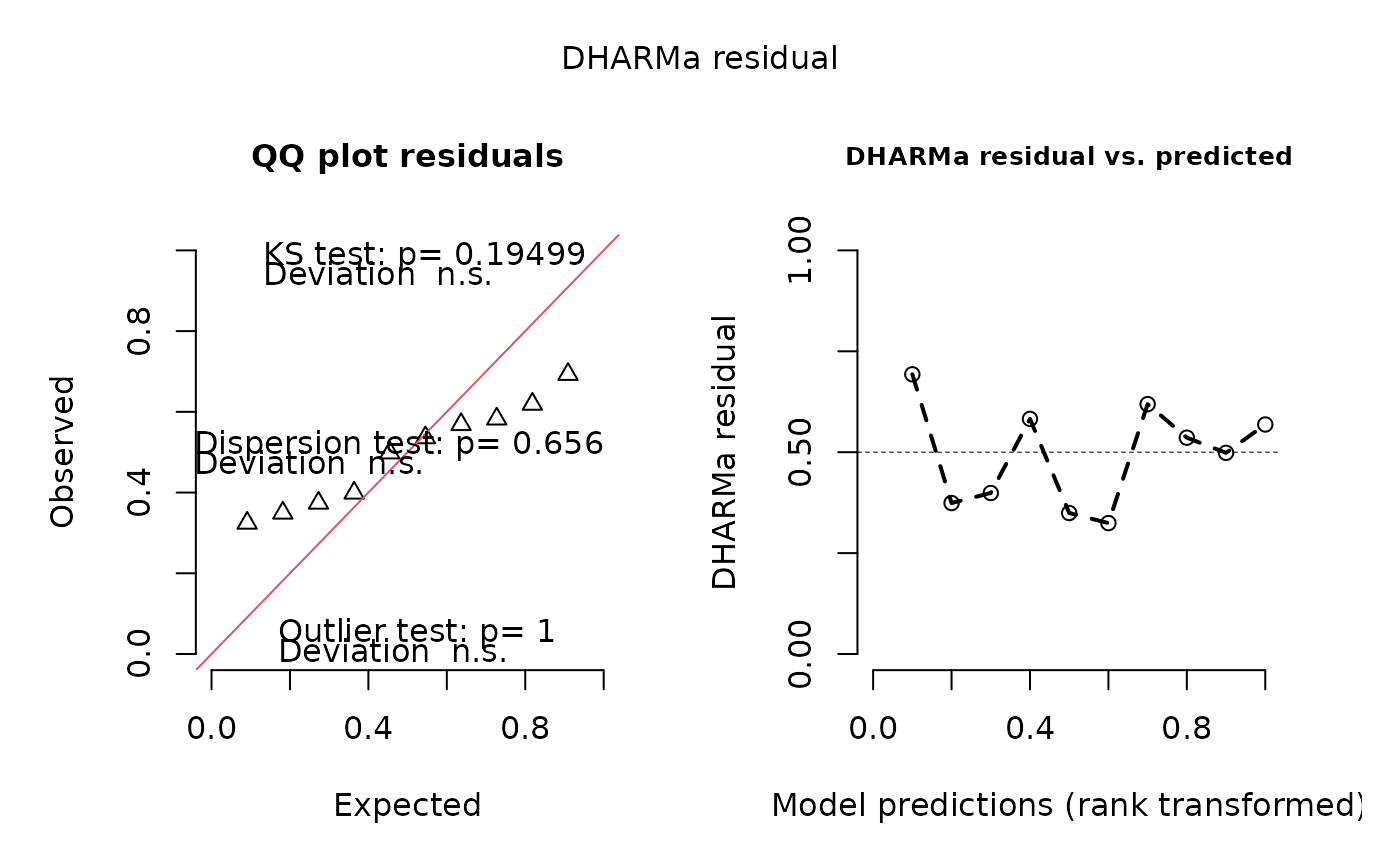 # we see one residual point per RE
# with group as variable in your environment
# but then you need to exclude NAs by hand
simulationOutput5 = recalculateResiduals(simulationOutput1, group = testData$group)
# calculating residuals only for subset of the data
simulationOutput6 = recalculateResiduals(simulationOutput1, sel = testData$group == 1)
plot(simulationOutput6, quantreg = FALSE)
# we see one residual point per RE
# with group as variable in your environment
# but then you need to exclude NAs by hand
simulationOutput5 = recalculateResiduals(simulationOutput1, group = testData$group)
# calculating residuals only for subset of the data
simulationOutput6 = recalculateResiduals(simulationOutput1, sel = testData$group == 1)
plot(simulationOutput6, quantreg = FALSE)
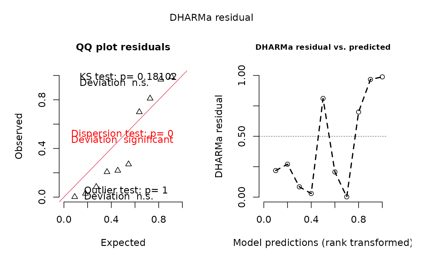 # or with sel as formula
simulationOutput7 = recalculateResiduals(simulationOutput1, sel = ~Environment1<0.5)
# as condition based on a variable in your environment
simulationOutput8 = recalculateResiduals(simulationOutput1, sel = testData$Environment1<0.5)
# or combine group and sel
simulationOutput9 = recalculateResiduals(simulationOutput1, group = ~group, sel = ~Environment1<0.5)
# or as subset of rows
# (note: order of rows is based on residuals, not on original dataframe)
# so be careful with NAs!
simulationOutput10 = recalculateResiduals(simulationOutput1, sel = 1:20)
# or with sel as formula
simulationOutput7 = recalculateResiduals(simulationOutput1, sel = ~Environment1<0.5)
# as condition based on a variable in your environment
simulationOutput8 = recalculateResiduals(simulationOutput1, sel = testData$Environment1<0.5)
# or combine group and sel
simulationOutput9 = recalculateResiduals(simulationOutput1, group = ~group, sel = ~Environment1<0.5)
# or as subset of rows
# (note: order of rows is based on residuals, not on original dataframe)
# so be careful with NAs!
simulationOutput10 = recalculateResiduals(simulationOutput1, sel = 1:20)