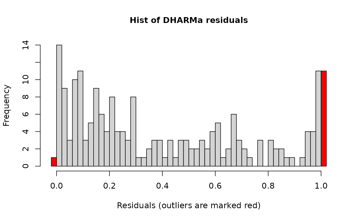
The function produces a histogram from a DHARMa output. Outliers are marked in red.
Details
The function calls hist() to create a histogram of the scaled residuals. Outliers are marked red as default but it can be changed by setting options(DHARMaSignalColor = "red") to a different color. See getOption("DHARMaSignalColor") for the current setting.
Examples
testData = createData(sampleSize = 200, family = poisson(),
fixedEffects = c(1,1),
randomEffectVariance = 1, numGroups = 10)
testData$Environment2[1] = NA
fittedModel <- glm(observedResponse ~ Environment1 + Environment2,
family = "poisson", data = testData)
simulationOutput <- simulateResiduals(fittedModel = fittedModel)
######### main plotting function #############
plot(simulationOutput)
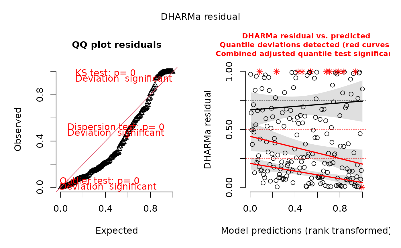 # for all functions, quantreg = T (default) will be more informative
# but slower. Alternative:
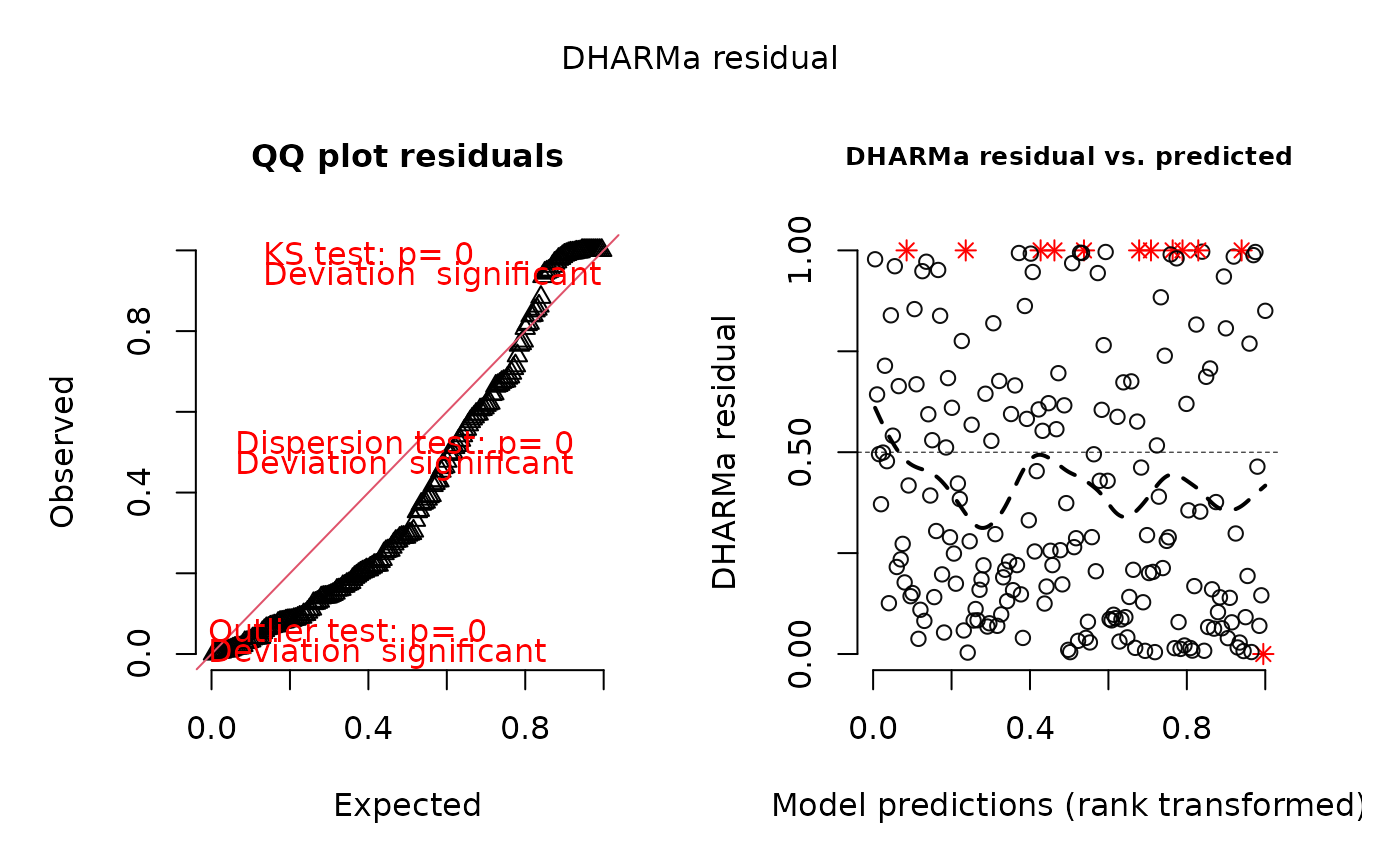
plot(simulationOutput, quantreg = FALSE)
# for all functions, quantreg = T (default) will be more informative
# but slower. Alternative:
plot(simulationOutput, quantreg = FALSE)
 ############# Distribution ######################
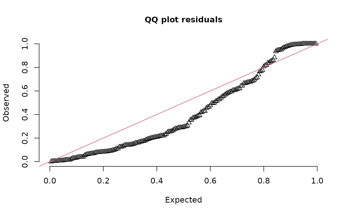
plotQQunif(simulationOutput = simulationOutput,
testDispersion = FALSE,
testUniformity = FALSE,
testOutliers = FALSE)
############# Distribution ######################
plotQQunif(simulationOutput = simulationOutput,
testDispersion = FALSE,
testUniformity = FALSE,
testOutliers = FALSE)
 hist(simulationOutput)