Doctoral Publications — PhDPublications • AER

Cross-section data on the scientific productivity of PhD students in biochemistry.

Usage

data("PhDPublications")

Format

A data frame containing 915 observations on 6 variables.

articles: Number of articles published during last 3 years of PhD.
gender: factor indicating gender.
married: factor. Is the PhD student married?
kids: Number of children less than 6 years old.
prestige: Prestige of the graduate program.
mentor: Number of articles published by student's mentor.

Source

Online complements to Long (1997).

References

Long, J.S. (1990). Regression Models for Categorical and Limited Dependent Variables. Thousand Oaks: Sage Publications.

Long, J.S. (1997). The Origin of Sex Differences in Science. Social Forces, 68, 1297–1315.

Examples

## from Long (1997)
data("PhDPublications")

## Table 8.1, p. 227
summary(PhDPublications)
#>     articles         gender    married        kids           prestige    
#>  Min.   : 0.000   male  :494   no :309   Min.   :0.0000   Min.   :0.755  
#>  1st Qu.: 0.000   female:421   yes:606   1st Qu.:0.0000   1st Qu.:2.260  
#>  Median : 1.000                          Median :0.0000   Median :3.150  
#>  Mean   : 1.693                          Mean   :0.4951   Mean   :3.103  
#>  3rd Qu.: 2.000                          3rd Qu.:1.0000   3rd Qu.:3.920  
#>  Max.   :19.000                          Max.   :3.0000   Max.   :4.620  
#>      mentor      
#>  Min.   : 0.000  
#>  1st Qu.: 3.000  
#>  Median : 6.000  
#>  Mean   : 8.767  
#>  3rd Qu.:12.000  
#>  Max.   :77.000  

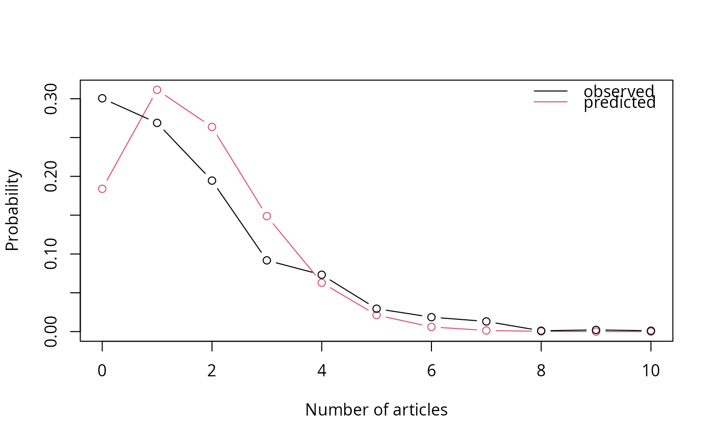
## Figure 8.2, p. 220
plot(0:10, dpois(0:10, mean(PhDPublications$articles)), type = "b", col = 2,
  xlab = "Number of articles", ylab = "Probability")
lines(0:10, prop.table(table(PhDPublications$articles))[1:11], type = "b")
legend("topright", c("observed", "predicted"), col = 1:2, lty = rep(1, 2), bty = "n")


## Table 8.2, p. 228
fm_lrm <- lm(log(articles + 0.5) ~ ., data = PhDPublications)
summary(fm_lrm)
#> 
#> Call:
#> lm(formula = log(articles + 0.5) ~ ., data = PhDPublications)
#> 
#> Residuals:
#>      Min       1Q   Median       3Q      Max 
#> -1.87006 -0.87012  0.07973  0.63630  2.17374 
#> 
#> Coefficients:
#>               Estimate Std. Error t value Pr(>|t|)    
#> (Intercept)   0.177774   0.107725   1.650   0.0992 .  
#> genderfemale -0.134567   0.057298  -2.349   0.0191 *  
#> marriedyes    0.132826   0.065027   2.043   0.0414 *  
#> kids         -0.133148   0.040655  -3.275   0.0011 ** 
#> prestige      0.025502   0.028469   0.896   0.3706    
#> mentor        0.025421   0.002954   8.607   <2e-16 ***
#> ---
#> Signif. codes:  0 ‘***’ 0.001 ‘**’ 0.01 ‘*’ 0.05 ‘.’ 0.1 ‘ ’ 1
#> 
#> Residual standard error: 0.8146 on 909 degrees of freedom
#> Multiple R-squared:  0.1008,	Adjusted R-squared:  0.09582 
#> F-statistic: 20.37 on 5 and 909 DF,  p-value: < 2.2e-16
#> 
-2 * logLik(fm_lrm)
#> 'log Lik.' 2215.323 (df=7)
fm_prm <- glm(articles ~ ., data = PhDPublications, family = poisson)
library("MASS")
fm_nbrm <- glm.nb(articles ~ ., data = PhDPublications)

## Table 8.3, p. 246
library("pscl")
fm_zip <- zeroinfl(articles ~ . | ., data = PhDPublications)
fm_zinb <- zeroinfl(articles ~ . | ., data = PhDPublications, dist = "negbin")