Demand for Medical Care in NMES 1988
NMES1988.RdCross-section data originating from the US National Medical Expenditure Survey (NMES) conducted in 1987 and 1988. The NMES is based upon a representative, national probability sample of the civilian non-institutionalized population and individuals admitted to long-term care facilities during 1987. The data are a subsample of individuals ages 66 and over all of whom are covered by Medicare (a public insurance program providing substantial protection against health-care costs).
Usage
data("NMES1988")Format
A data frame containing 4,406 observations on 19 variables.
- visits
Number of physician office visits.
- nvisits
Number of non-physician office visits.
- ovisits
Number of physician hospital outpatient visits.
- novisits
Number of non-physician hospital outpatient visits.
- emergency
Emergency room visits.
- hospital
Number of hospital stays.
- health
Factor indicating self-perceived health status, levels are
"poor","average"(reference category),"excellent".- chronic
Number of chronic conditions.
- adl
Factor indicating whether the individual has a condition that limits activities of daily living (
"limited") or not ("normal").- region
Factor indicating region, levels are
northeast,midwest,west,other(reference category).- age
Age in years (divided by 10).
- afam
Factor. Is the individual African-American?
- gender
Factor indicating gender.
- married
Factor. is the individual married?
- school
Number of years of education.
- income
Family income in USD 10,000.
- employed
Factor. Is the individual employed?
- insurance
Factor. Is the individual covered by private insurance?
- medicaid
Factor. Is the individual covered by Medicaid?
References
Cameron, A.C. and Trivedi, P.K. (1998). Regression Analysis of Count Data. Cambridge: Cambridge University Press.
Deb, P., and Trivedi, P.K. (1997). Demand for Medical Care by the Elderly: A Finite Mixture Approach. Journal of Applied Econometrics, 12, 313–336.
Zeileis, A., Kleiber, C., and Jackman, S. (2008). Regression Models for Count Data in R. Journal of Statistical Software, 27(8). doi:10.18637/jss.v027.i08 .
Examples
## packages
library("MASS")
library("pscl")
## select variables for analysis
data("NMES1988")
nmes <- NMES1988[, c(1, 7:8, 13, 15, 18)]
## dependent variable
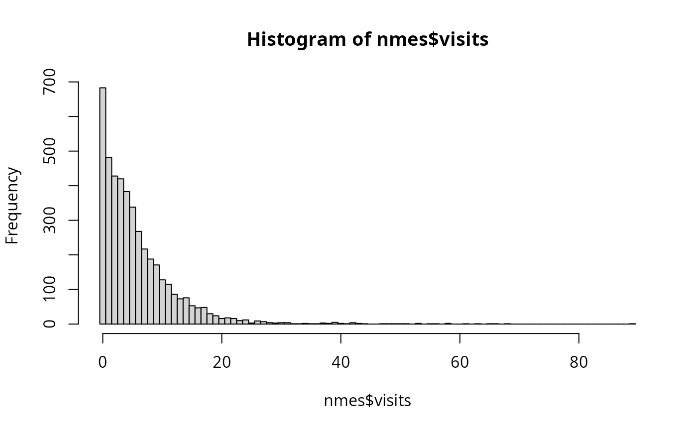
hist(nmes$visits, breaks = 0:(max(nmes$visits)+1) - 0.5)
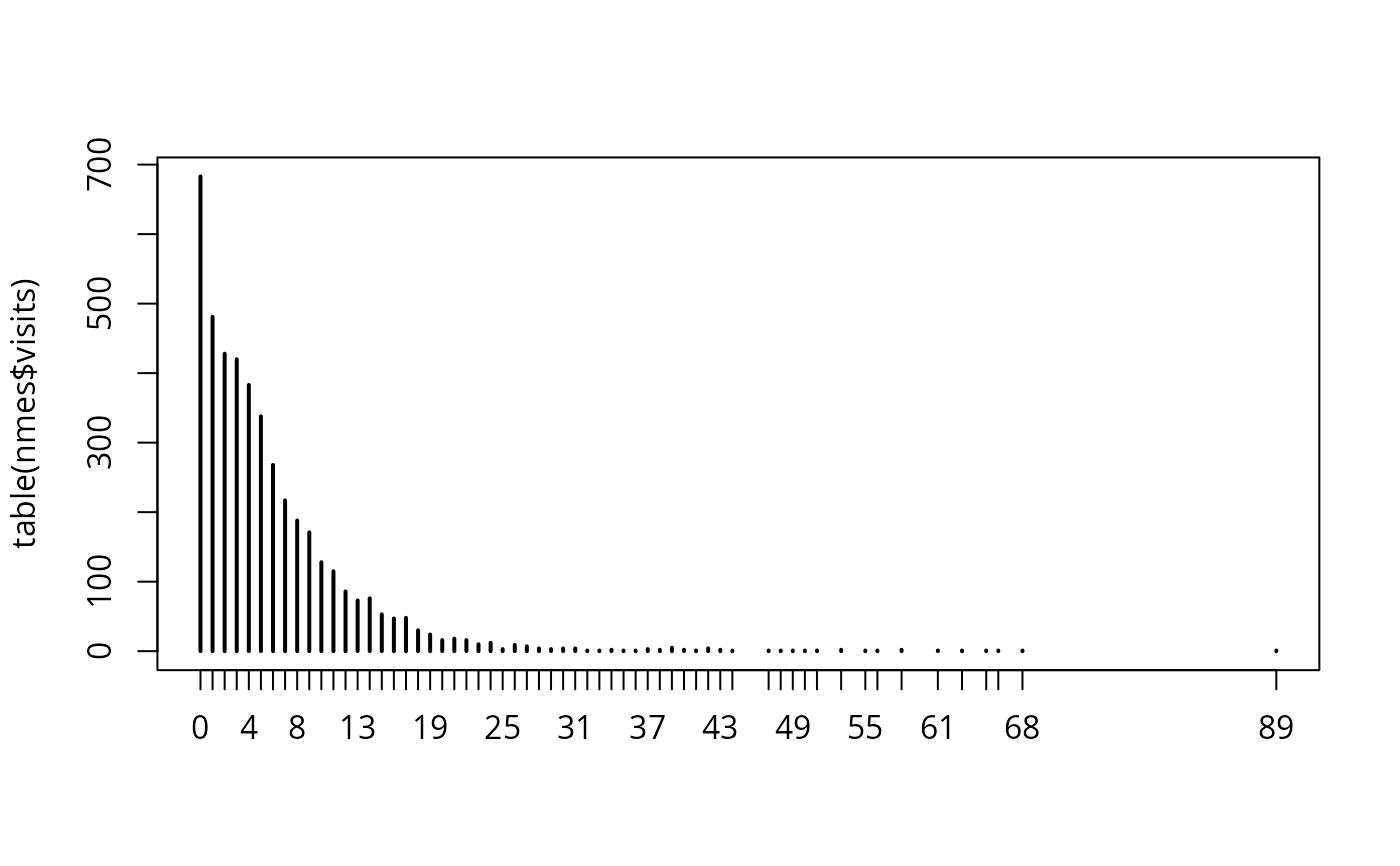
 plot(table(nmes$visits))
 ## convenience transformations for exploratory graphics
clog <- function(x) log(x + 0.5)
cfac <- function(x, breaks = NULL) {
if(is.null(breaks)) breaks <- unique(quantile(x, 0:10/10))
x <- cut(x, breaks, include.lowest = TRUE, right = FALSE)
levels(x) <- paste(breaks[-length(breaks)], ifelse(diff(breaks) > 1,
c(paste("-", breaks[-c(1, length(breaks))] - 1, sep = ""), "+"), ""), sep = "")
return(x)
}
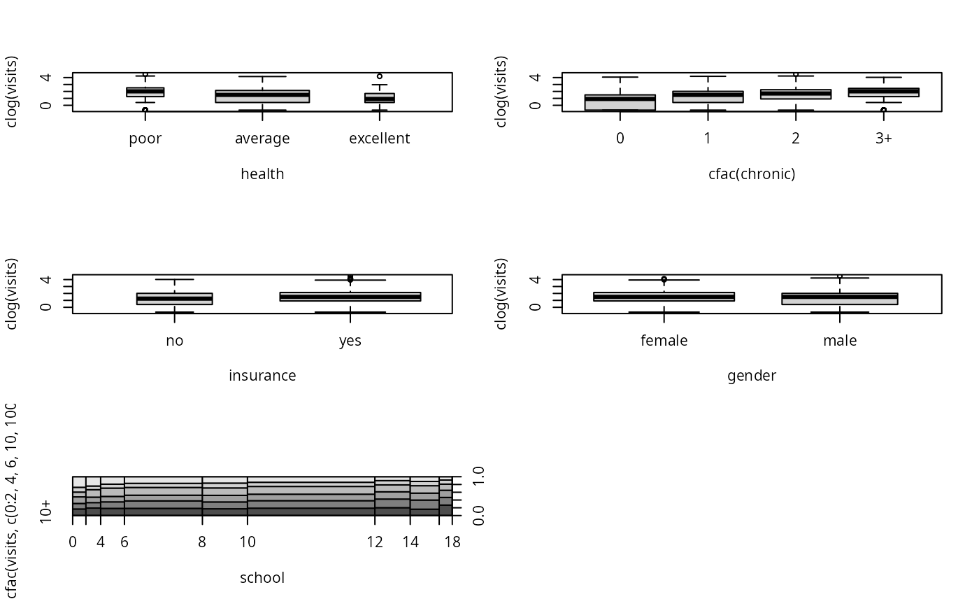
## bivariate visualization
par(mfrow = c(3, 2))
plot(clog(visits) ~ health, data = nmes, varwidth = TRUE)
plot(clog(visits) ~ cfac(chronic), data = nmes)
plot(clog(visits) ~ insurance, data = nmes, varwidth = TRUE)
plot(clog(visits) ~ gender, data = nmes, varwidth = TRUE)
plot(cfac(visits, c(0:2, 4, 6, 10, 100)) ~ school, data = nmes, breaks = 9)
par(mfrow = c(1, 1))
## convenience transformations for exploratory graphics
clog <- function(x) log(x + 0.5)
cfac <- function(x, breaks = NULL) {
if(is.null(breaks)) breaks <- unique(quantile(x, 0:10/10))
x <- cut(x, breaks, include.lowest = TRUE, right = FALSE)
levels(x) <- paste(breaks[-length(breaks)], ifelse(diff(breaks) > 1,
c(paste("-", breaks[-c(1, length(breaks))] - 1, sep = ""), "+"), ""), sep = "")
return(x)
}
## bivariate visualization
par(mfrow = c(3, 2))
plot(clog(visits) ~ health, data = nmes, varwidth = TRUE)
plot(clog(visits) ~ cfac(chronic), data = nmes)
plot(clog(visits) ~ insurance, data = nmes, varwidth = TRUE)
plot(clog(visits) ~ gender, data = nmes, varwidth = TRUE)
plot(cfac(visits, c(0:2, 4, 6, 10, 100)) ~ school, data = nmes, breaks = 9)
par(mfrow = c(1, 1))
 ## Poisson regression
nmes_pois <- glm(visits ~ ., data = nmes, family = poisson)
summary(nmes_pois)
#>
#> Call:
#> glm(formula = visits ~ ., family = poisson, data = nmes)
#>
#> Coefficients:
#> Estimate Std. Error z value Pr(>|z|)
#> (Intercept) 1.034542 0.023857 43.364 <2e-16 ***
#> healthpoor 0.318205 0.017479 18.205 <2e-16 ***
#> healthexcellent -0.379045 0.030291 -12.514 <2e-16 ***
#> chronic 0.168793 0.004471 37.755 <2e-16 ***
#> gendermale -0.108014 0.012943 -8.346 <2e-16 ***
#> school 0.025754 0.001843 13.972 <2e-16 ***
#> insuranceyes 0.216007 0.016872 12.803 <2e-16 ***
#> ---
#> Signif. codes: 0 ‘***’ 0.001 ‘**’ 0.01 ‘*’ 0.05 ‘.’ 0.1 ‘ ’ 1
#>
#> (Dispersion parameter for poisson family taken to be 1)
#>
#> Null deviance: 26943 on 4405 degrees of freedom
#> Residual deviance: 23808 on 4399 degrees of freedom
#> AIC: 36597
#>
#> Number of Fisher Scoring iterations: 5
#>
## LM test for overdispersion
dispersiontest(nmes_pois)
#>
#> Overdispersion test
#>
#> data: nmes_pois
#> z = 11.557, p-value < 2.2e-16
#> alternative hypothesis: true dispersion is greater than 1
#> sample estimates:
#> dispersion
#> 6.976619
#>
dispersiontest(nmes_pois, trafo = 2)
#>
#> Overdispersion test
#>
#> data: nmes_pois
#> z = 11.307, p-value < 2.2e-16
#> alternative hypothesis: true alpha is greater than 0
#> sample estimates:
#> alpha
#> 0.9497124
#>
## sandwich covariance matrix
coeftest(nmes_pois, vcov = sandwich)
#>
#> z test of coefficients:
#>
#> Estimate Std. Error z value Pr(>|z|)
#> (Intercept) 1.0345418 0.0648436 15.9544 < 2.2e-16 ***
#> healthpoor 0.3182048 0.0555787 5.7253 1.032e-08 ***
#> healthexcellent -0.3790454 0.0777311 -4.8764 1.081e-06 ***
#> chronic 0.1687932 0.0121860 13.8514 < 2.2e-16 ***
#> gendermale -0.1080145 0.0357357 -3.0226 0.002506 **
#> school 0.0257542 0.0051316 5.0187 5.202e-07 ***
#> insuranceyes 0.2160070 0.0430293 5.0200 5.167e-07 ***
#> ---
#> Signif. codes: 0 ‘***’ 0.001 ‘**’ 0.01 ‘*’ 0.05 ‘.’ 0.1 ‘ ’ 1
#>
## quasipoisson model
nmes_qpois <- glm(visits ~ ., data = nmes, family = quasipoisson)
## NegBin regression
nmes_nb <- glm.nb(visits ~ ., data = nmes)
## hurdle regression
nmes_hurdle <- hurdle(visits ~ . | chronic + insurance + school + gender,
data = nmes, dist = "negbin")
## zero-inflated regression model
nmes_zinb <- zeroinfl(visits ~ . | chronic + insurance + school + gender,
data = nmes, dist = "negbin")
## compare estimated coefficients
fm <- list("ML-Pois" = nmes_pois, "Quasi-Pois" = nmes_qpois, "NB" = nmes_nb,
"Hurdle-NB" = nmes_hurdle, "ZINB" = nmes_zinb)
round(sapply(fm, function(x) coef(x)[1:7]), digits = 3)
#> ML-Pois Quasi-Pois NB Hurdle-NB ZINB
#> (Intercept) 1.035 1.035 0.940 1.194 1.198
#> healthpoor 0.318 0.318 0.368 0.383 0.349
#> healthexcellent -0.379 -0.379 -0.374 -0.368 -0.354
#> chronic 0.169 0.169 0.196 0.148 0.150
#> gendermale -0.108 -0.108 -0.115 -0.056 -0.072
#> school 0.026 0.026 0.027 0.021 0.022
#> insuranceyes 0.216 0.216 0.250 0.130 0.151
## associated standard errors
round(cbind("ML-Pois" = sqrt(diag(vcov(nmes_pois))),
"Adj-Pois" = sqrt(diag(sandwich(nmes_pois))),
sapply(fm[-1], function(x) sqrt(diag(vcov(x)))[1:7])),
digits = 3)
#> ML-Pois Adj-Pois Quasi-Pois NB Hurdle-NB ZINB
#> (Intercept) 0.024 0.065 0.063 0.055 0.060 0.057
#> healthpoor 0.017 0.056 0.046 0.049 0.049 0.046
#> healthexcellent 0.030 0.078 0.080 0.062 0.067 0.061
#> chronic 0.004 0.012 0.012 0.012 0.013 0.012
#> gendermale 0.013 0.036 0.034 0.032 0.033 0.032
#> school 0.002 0.005 0.005 0.004 0.005 0.004
#> insuranceyes 0.017 0.043 0.045 0.040 0.044 0.042
## log-likelihoods and number of estimated parameters
rbind(logLik = sapply(fm, function(x) round(logLik(x), digits = 0)),
Df = sapply(fm, function(x) attr(logLik(x), "df")))
#> ML-Pois Quasi-Pois NB Hurdle-NB ZINB
#> logLik -18291 NA -12227 -12153 -12155
#> Df 7 8 8 13 13
## predicted number of zeros
round(c("Obs" = sum(nmes$visits < 1),
"ML-Pois" = sum(dpois(0, fitted(nmes_pois))),
"Adj-Pois" = NA,
"Quasi-Pois" = NA,
"NB" = sum(dnbinom(0, mu = fitted(nmes_nb), size = nmes_nb$theta)),
"NB-Hurdle" = sum(predict(nmes_hurdle, type = "prob")[,1]),
"ZINB" = sum(predict(nmes_zinb, type = "prob")[,1])))
#> Obs ML-Pois Adj-Pois Quasi-Pois NB NB-Hurdle ZINB
#> 683 46 NA NA 618 683 712
## coefficients of zero-augmentation models
t(sapply(fm[4:5], function(x) round(x$coefficients$zero, digits = 3)))
#> (Intercept) chronic insuranceyes school gendermale
#> Hurdle-NB 0.054 0.577 0.742 0.056 -0.406
#> ZINB -0.098 -1.302 -1.193 -0.087 0.583
## Poisson regression
nmes_pois <- glm(visits ~ ., data = nmes, family = poisson)
summary(nmes_pois)
#>
#> Call:
#> glm(formula = visits ~ ., family = poisson, data = nmes)
#>
#> Coefficients:
#> Estimate Std. Error z value Pr(>|z|)
#> (Intercept) 1.034542 0.023857 43.364 <2e-16 ***
#> healthpoor 0.318205 0.017479 18.205 <2e-16 ***
#> healthexcellent -0.379045 0.030291 -12.514 <2e-16 ***
#> chronic 0.168793 0.004471 37.755 <2e-16 ***
#> gendermale -0.108014 0.012943 -8.346 <2e-16 ***
#> school 0.025754 0.001843 13.972 <2e-16 ***
#> insuranceyes 0.216007 0.016872 12.803 <2e-16 ***
#> ---
#> Signif. codes: 0 ‘***’ 0.001 ‘**’ 0.01 ‘*’ 0.05 ‘.’ 0.1 ‘ ’ 1
#>
#> (Dispersion parameter for poisson family taken to be 1)
#>
#> Null deviance: 26943 on 4405 degrees of freedom
#> Residual deviance: 23808 on 4399 degrees of freedom
#> AIC: 36597
#>
#> Number of Fisher Scoring iterations: 5
#>
## LM test for overdispersion
dispersiontest(nmes_pois)
#>
#> Overdispersion test
#>
#> data: nmes_pois
#> z = 11.557, p-value < 2.2e-16
#> alternative hypothesis: true dispersion is greater than 1
#> sample estimates:
#> dispersion
#> 6.976619
#>
dispersiontest(nmes_pois, trafo = 2)
#>
#> Overdispersion test
#>
#> data: nmes_pois
#> z = 11.307, p-value < 2.2e-16
#> alternative hypothesis: true alpha is greater than 0
#> sample estimates:
#> alpha
#> 0.9497124
#>
## sandwich covariance matrix
coeftest(nmes_pois, vcov = sandwich)
#>
#> z test of coefficients:
#>
#> Estimate Std. Error z value Pr(>|z|)
#> (Intercept) 1.0345418 0.0648436 15.9544 < 2.2e-16 ***
#> healthpoor 0.3182048 0.0555787 5.7253 1.032e-08 ***
#> healthexcellent -0.3790454 0.0777311 -4.8764 1.081e-06 ***
#> chronic 0.1687932 0.0121860 13.8514 < 2.2e-16 ***
#> gendermale -0.1080145 0.0357357 -3.0226 0.002506 **
#> school 0.0257542 0.0051316 5.0187 5.202e-07 ***
#> insuranceyes 0.2160070 0.0430293 5.0200 5.167e-07 ***
#> ---
#> Signif. codes: 0 ‘***’ 0.001 ‘**’ 0.01 ‘*’ 0.05 ‘.’ 0.1 ‘ ’ 1
#>
## quasipoisson model
nmes_qpois <- glm(visits ~ ., data = nmes, family = quasipoisson)
## NegBin regression
nmes_nb <- glm.nb(visits ~ ., data = nmes)
## hurdle regression
nmes_hurdle <- hurdle(visits ~ . | chronic + insurance + school + gender,
data = nmes, dist = "negbin")
## zero-inflated regression model
nmes_zinb <- zeroinfl(visits ~ . | chronic + insurance + school + gender,
data = nmes, dist = "negbin")
## compare estimated coefficients
fm <- list("ML-Pois" = nmes_pois, "Quasi-Pois" = nmes_qpois, "NB" = nmes_nb,
"Hurdle-NB" = nmes_hurdle, "ZINB" = nmes_zinb)
round(sapply(fm, function(x) coef(x)[1:7]), digits = 3)
#> ML-Pois Quasi-Pois NB Hurdle-NB ZINB
#> (Intercept) 1.035 1.035 0.940 1.194 1.198
#> healthpoor 0.318 0.318 0.368 0.383 0.349
#> healthexcellent -0.379 -0.379 -0.374 -0.368 -0.354
#> chronic 0.169 0.169 0.196 0.148 0.150
#> gendermale -0.108 -0.108 -0.115 -0.056 -0.072
#> school 0.026 0.026 0.027 0.021 0.022
#> insuranceyes 0.216 0.216 0.250 0.130 0.151
## associated standard errors
round(cbind("ML-Pois" = sqrt(diag(vcov(nmes_pois))),
"Adj-Pois" = sqrt(diag(sandwich(nmes_pois))),
sapply(fm[-1], function(x) sqrt(diag(vcov(x)))[1:7])),
digits = 3)
#> ML-Pois Adj-Pois Quasi-Pois NB Hurdle-NB ZINB
#> (Intercept) 0.024 0.065 0.063 0.055 0.060 0.057
#> healthpoor 0.017 0.056 0.046 0.049 0.049 0.046
#> healthexcellent 0.030 0.078 0.080 0.062 0.067 0.061
#> chronic 0.004 0.012 0.012 0.012 0.013 0.012
#> gendermale 0.013 0.036 0.034 0.032 0.033 0.032
#> school 0.002 0.005 0.005 0.004 0.005 0.004
#> insuranceyes 0.017 0.043 0.045 0.040 0.044 0.042
## log-likelihoods and number of estimated parameters
rbind(logLik = sapply(fm, function(x) round(logLik(x), digits = 0)),
Df = sapply(fm, function(x) attr(logLik(x), "df")))
#> ML-Pois Quasi-Pois NB Hurdle-NB ZINB
#> logLik -18291 NA -12227 -12153 -12155
#> Df 7 8 8 13 13
## predicted number of zeros
round(c("Obs" = sum(nmes$visits < 1),
"ML-Pois" = sum(dpois(0, fitted(nmes_pois))),
"Adj-Pois" = NA,
"Quasi-Pois" = NA,
"NB" = sum(dnbinom(0, mu = fitted(nmes_nb), size = nmes_nb$theta)),
"NB-Hurdle" = sum(predict(nmes_hurdle, type = "prob")[,1]),
"ZINB" = sum(predict(nmes_zinb, type = "prob")[,1])))
#> Obs ML-Pois Adj-Pois Quasi-Pois NB NB-Hurdle ZINB
#> 683 46 NA NA 618 683 712
## coefficients of zero-augmentation models
t(sapply(fm[4:5], function(x) round(x$coefficients$zero, digits = 3)))
#> (Intercept) chronic insuranceyes school gendermale
#> Hurdle-NB 0.054 0.577 0.742 0.056 -0.406
#> ZINB -0.098 -1.302 -1.193 -0.087 0.583