MSCI Switzerland Index
MSCISwitzerland.RdTime series of the MSCI Switzerland index.
Usage
data("MSCISwitzerland")Format
A daily univariate time series from 1994-12-30 to 2012-12-31 (of class "zoo" with "Date" index).
References
Ding, Z., Granger, C. W. J. and Engle, R. F. (1993). A Long Memory Property of Stock Market Returns and a New Model. Journal of Empirical Finance, 1(1), 83–106.
Franses, P.H., van Dijk, D. and Opschoor, A. (2014). Time Series Models for Business and Economic Forecasting, 2nd ed. Cambridge, UK: Cambridge University Press.
Examples
#> Loading required namespace: fGarch
#> Loading required namespace: rugarch
data("MSCISwitzerland", package = "AER")
## p.190, Fig. 7.6
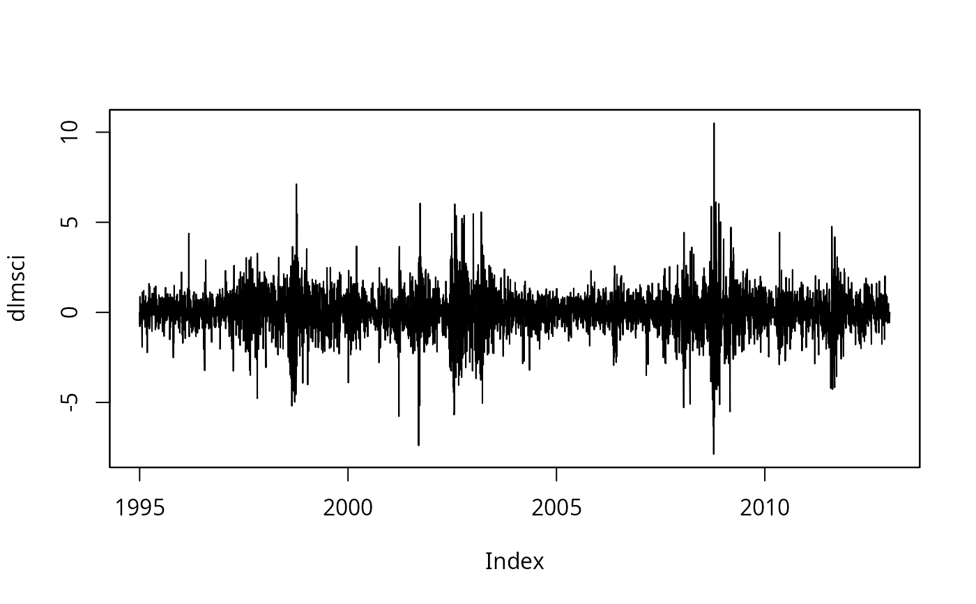
dlmsci <- 100 * diff(log(MSCISwitzerland))
plot(dlmsci)
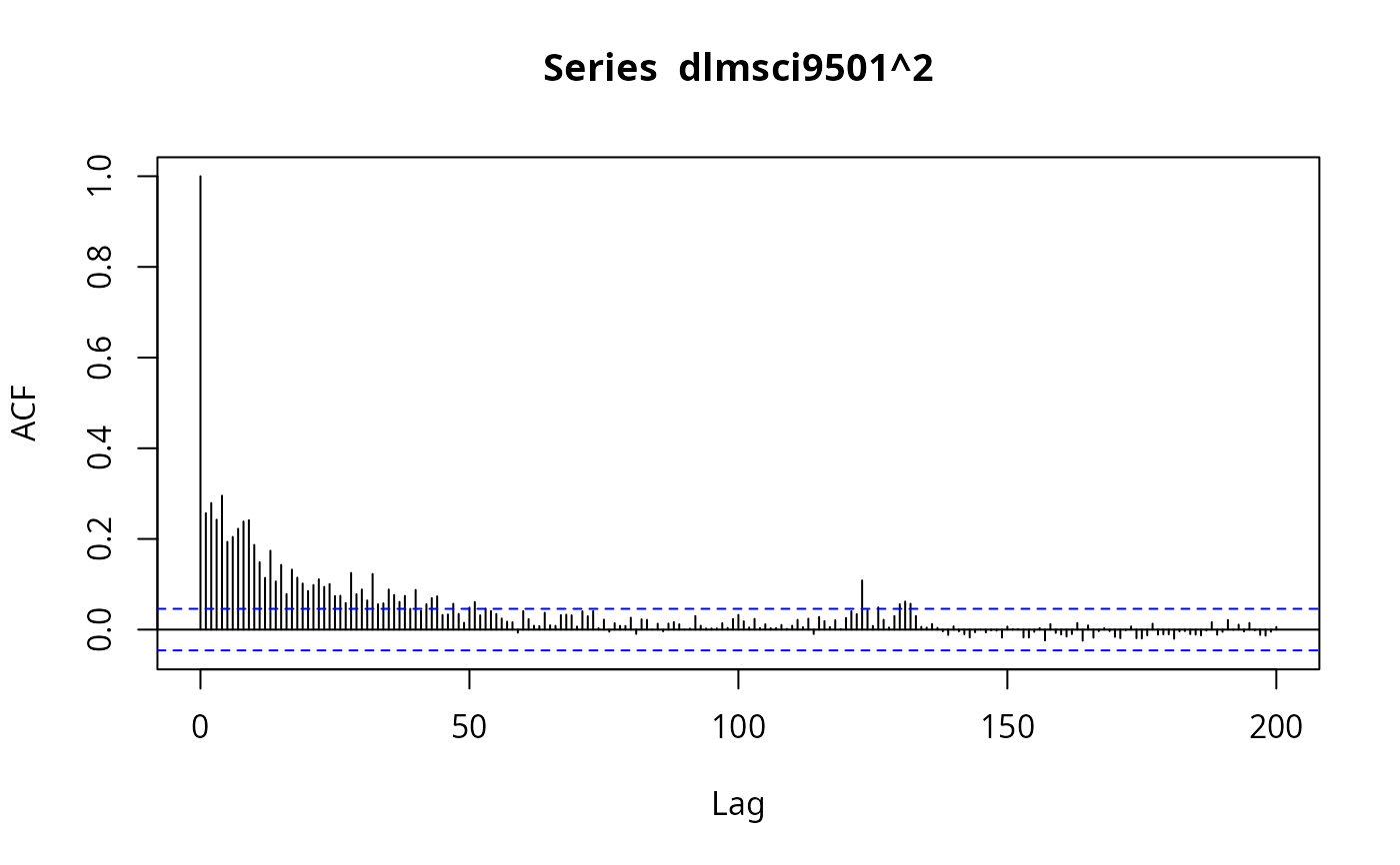
 dlmsci9501 <- window(dlmsci, end = as.Date("2001-12-31"))
## Figure 7.7
plot(acf(dlmsci9501^2, lag.max = 200, na.action = na.exclude),
ylim = c(-0.1, 0.3), type = "l")
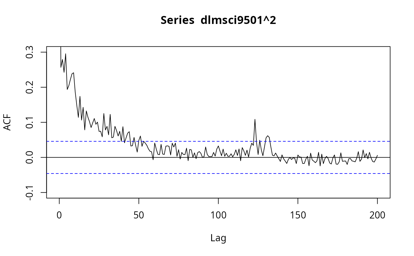
dlmsci9501 <- window(dlmsci, end = as.Date("2001-12-31"))
## Figure 7.7
plot(acf(dlmsci9501^2, lag.max = 200, na.action = na.exclude),
ylim = c(-0.1, 0.3), type = "l")
 ## GARCH(1,1) model, p.190, eq. (7.60)
## standard errors using first derivatives (as apparently used by Franses et al.)
library("tseries")
msci9501_g11 <- garch(zooreg(dlmsci9501), trace = FALSE)
summary(msci9501_g11)
#>
#> Call:
#> garch(x = zooreg(dlmsci9501), trace = FALSE)
#>
#> Model:
#> GARCH(1,1)
#>
#> Residuals:
#> Min 1Q Median 3Q Max
#> -5.30570 -0.50860 0.05433 0.68275 5.71286
#>
#> Coefficient(s):
#> Estimate Std. Error t value Pr(>|t|)
#> a0 0.039017 0.007657 5.096 3.48e-07 ***
#> a1 0.115525 0.011968 9.653 < 2e-16 ***
#> b1 0.853031 0.016621 51.323 < 2e-16 ***
#> ---
#> Signif. codes: 0 ‘***’ 0.001 ‘**’ 0.01 ‘*’ 0.05 ‘.’ 0.1 ‘ ’ 1
#>
#> Diagnostic Tests:
#> Jarque Bera Test
#>
#> data: Residuals
#> X-squared = 322.29, df = 2, p-value < 2.2e-16
#>
#>
#> Box-Ljung test
#>
#> data: Squared.Residuals
#> X-squared = 0.74665, df = 1, p-value = 0.3875
#>
## standard errors using second derivatives
library("fGarch")
#> NOTE: Packages 'fBasics', 'timeDate', and 'timeSeries' are no longer
#> attached to the search() path when 'fGarch' is attached.
#>
#> If needed attach them yourself in your R script by e.g.,
#> require("timeSeries")
msci9501_g11a <- garchFit( ~ garch(1,1), include.mean = FALSE,
data = dlmsci9501, trace = FALSE)
summary(msci9501_g11a)
#>
#> Title:
#> GARCH Modelling
#>
#> Call:
#> garchFit(formula = ~garch(1, 1), data = dlmsci9501, include.mean = FALSE,
#> trace = FALSE)
#>
#> Mean and Variance Equation:
#> data ~ garch(1, 1)
#> <environment: 0x5bb5ed622368>
#> [data = dlmsci9501]
#>
#> Conditional Distribution:
#> norm
#>
#> Coefficient(s):
#> omega alpha1 beta1
#> 0.039178 0.115480 0.852834
#>
#> Std. Errors:
#> based on Hessian
#>
#> Error Analysis:
#> Estimate Std. Error t value Pr(>|t|)
#> omega 0.039178 0.009849 3.978 6.96e-05 ***
#> alpha1 0.115480 0.016283 7.092 1.32e-12 ***
#> beta1 0.852834 0.020529 41.543 < 2e-16 ***
#> ---
#> Signif. codes: 0 ‘***’ 0.001 ‘**’ 0.01 ‘*’ 0.05 ‘.’ 0.1 ‘ ’ 1
#>
#> Log Likelihood:
#> -2566.521 normalized: -1.405543
#>
#> Description:
#> Wed Feb 18 21:33:14 2026 by user: andrew
#>
#>
#>
#> Standardised Residuals Tests:
#> Statistic p-Value
#> Jarque-Bera Test R Chi^2 322.9213582 0.000000e+00
#> Shapiro-Wilk Test R W 0.9811351 8.649613e-15
#> Ljung-Box Test R Q(10) 18.7534129 4.350883e-02
#> Ljung-Box Test R Q(15) 20.5383235 1.522397e-01
#> Ljung-Box Test R Q(20) 24.3476524 2.275358e-01
#> Ljung-Box Test R^2 Q(10) 3.4624434 9.683582e-01
#> Ljung-Box Test R^2 Q(15) 5.9656935 9.803183e-01
#> Ljung-Box Test R^2 Q(20) 9.6069360 9.747523e-01
#> LM Arch Test R TR^2 5.3071118 9.469268e-01
#>
#> Information Criterion Statistics:
#> AIC BIC SIC HQIC
#> 2.814372 2.823424 2.814366 2.817711
#>
round(msci9501_g11a@fit$coef, 3)
#> omega alpha1 beta1
#> 0.039 0.115 0.853
round(msci9501_g11a@fit$se.coef, 3)
#> omega alpha1 beta1
#> 0.010 0.016 0.021
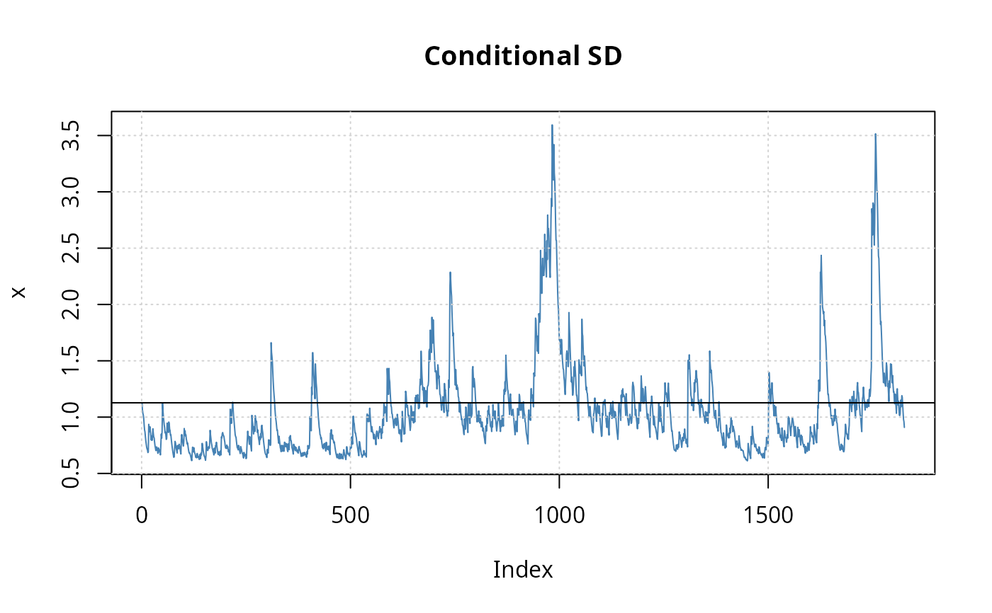
## Fig. 7.8, p.192
plot(msci9501_g11a, which = 2)
abline(h = sd(dlmsci9501))
## GARCH(1,1) model, p.190, eq. (7.60)
## standard errors using first derivatives (as apparently used by Franses et al.)
library("tseries")
msci9501_g11 <- garch(zooreg(dlmsci9501), trace = FALSE)
summary(msci9501_g11)
#>
#> Call:
#> garch(x = zooreg(dlmsci9501), trace = FALSE)
#>
#> Model:
#> GARCH(1,1)
#>
#> Residuals:
#> Min 1Q Median 3Q Max
#> -5.30570 -0.50860 0.05433 0.68275 5.71286
#>
#> Coefficient(s):
#> Estimate Std. Error t value Pr(>|t|)
#> a0 0.039017 0.007657 5.096 3.48e-07 ***
#> a1 0.115525 0.011968 9.653 < 2e-16 ***
#> b1 0.853031 0.016621 51.323 < 2e-16 ***
#> ---
#> Signif. codes: 0 ‘***’ 0.001 ‘**’ 0.01 ‘*’ 0.05 ‘.’ 0.1 ‘ ’ 1
#>
#> Diagnostic Tests:
#> Jarque Bera Test
#>
#> data: Residuals
#> X-squared = 322.29, df = 2, p-value < 2.2e-16
#>
#>
#> Box-Ljung test
#>
#> data: Squared.Residuals
#> X-squared = 0.74665, df = 1, p-value = 0.3875
#>
## standard errors using second derivatives
library("fGarch")
#> NOTE: Packages 'fBasics', 'timeDate', and 'timeSeries' are no longer
#> attached to the search() path when 'fGarch' is attached.
#>
#> If needed attach them yourself in your R script by e.g.,
#> require("timeSeries")
msci9501_g11a <- garchFit( ~ garch(1,1), include.mean = FALSE,
data = dlmsci9501, trace = FALSE)
summary(msci9501_g11a)
#>
#> Title:
#> GARCH Modelling
#>
#> Call:
#> garchFit(formula = ~garch(1, 1), data = dlmsci9501, include.mean = FALSE,
#> trace = FALSE)
#>
#> Mean and Variance Equation:
#> data ~ garch(1, 1)
#> <environment: 0x5bb5ed622368>
#> [data = dlmsci9501]
#>
#> Conditional Distribution:
#> norm
#>
#> Coefficient(s):
#> omega alpha1 beta1
#> 0.039178 0.115480 0.852834
#>
#> Std. Errors:
#> based on Hessian
#>
#> Error Analysis:
#> Estimate Std. Error t value Pr(>|t|)
#> omega 0.039178 0.009849 3.978 6.96e-05 ***
#> alpha1 0.115480 0.016283 7.092 1.32e-12 ***
#> beta1 0.852834 0.020529 41.543 < 2e-16 ***
#> ---
#> Signif. codes: 0 ‘***’ 0.001 ‘**’ 0.01 ‘*’ 0.05 ‘.’ 0.1 ‘ ’ 1
#>
#> Log Likelihood:
#> -2566.521 normalized: -1.405543
#>
#> Description:
#> Wed Feb 18 21:33:14 2026 by user: andrew
#>
#>
#>
#> Standardised Residuals Tests:
#> Statistic p-Value
#> Jarque-Bera Test R Chi^2 322.9213582 0.000000e+00
#> Shapiro-Wilk Test R W 0.9811351 8.649613e-15
#> Ljung-Box Test R Q(10) 18.7534129 4.350883e-02
#> Ljung-Box Test R Q(15) 20.5383235 1.522397e-01
#> Ljung-Box Test R Q(20) 24.3476524 2.275358e-01
#> Ljung-Box Test R^2 Q(10) 3.4624434 9.683582e-01
#> Ljung-Box Test R^2 Q(15) 5.9656935 9.803183e-01
#> Ljung-Box Test R^2 Q(20) 9.6069360 9.747523e-01
#> LM Arch Test R TR^2 5.3071118 9.469268e-01
#>
#> Information Criterion Statistics:
#> AIC BIC SIC HQIC
#> 2.814372 2.823424 2.814366 2.817711
#>
round(msci9501_g11a@fit$coef, 3)
#> omega alpha1 beta1
#> 0.039 0.115 0.853
round(msci9501_g11a@fit$se.coef, 3)
#> omega alpha1 beta1
#> 0.010 0.016 0.021
## Fig. 7.8, p.192
plot(msci9501_g11a, which = 2)
abline(h = sd(dlmsci9501))
 ## TGARCH model (also known as GJR-GARCH model), p. 191, eq. (7.61)
msci9501_tg11 <- garchFit( ~ aparch(1,1), include.mean = FALSE,
include.delta = FALSE, delta = 2, data = dlmsci9501, trace = FALSE)
summary(msci9501_tg11)
#>
#> Title:
#> GARCH Modelling
#>
#> Call:
#> garchFit(formula = ~aparch(1, 1), data = dlmsci9501, delta = 2,
#> include.mean = FALSE, include.delta = FALSE, trace = FALSE)
#>
#> Mean and Variance Equation:
#> data ~ aparch(1, 1)
#> <environment: 0x5bb5eb71b198>
#> [data = dlmsci9501]
#>
#> Conditional Distribution:
#> norm
#>
#> Coefficient(s):
#> omega alpha1 gamma1 beta1
#> 0.050659 0.085286 0.427898 0.856101
#>
#> Std. Errors:
#> based on Hessian
#>
#> Error Analysis:
#> Estimate Std. Error t value Pr(>|t|)
#> omega 0.05066 0.01180 4.293 1.76e-05 ***
#> alpha1 0.08529 0.01767 4.825 1.40e-06 ***
#> gamma1 0.42790 0.09671 4.425 9.66e-06 ***
#> beta1 0.85610 0.02348 36.463 < 2e-16 ***
#> ---
#> Signif. codes: 0 ‘***’ 0.001 ‘**’ 0.01 ‘*’ 0.05 ‘.’ 0.1 ‘ ’ 1
#>
#> Log Likelihood:
#> -2544.281 normalized: -1.393363
#>
#> Description:
#> Wed Feb 18 21:33:14 2026 by user: andrew
#>
#>
#>
#> Standardised Residuals Tests:
#> Statistic p-Value
#> Jarque-Bera Test R Chi^2 301.5135428 0.000000e+00
#> Shapiro-Wilk Test R W 0.9829266 6.022347e-14
#> Ljung-Box Test R Q(10) 21.5068487 1.782377e-02
#> Ljung-Box Test R Q(15) 23.6240653 7.175874e-02
#> Ljung-Box Test R Q(20) 27.8841646 1.121699e-01
#> Ljung-Box Test R^2 Q(10) 3.9434228 9.498632e-01
#> Ljung-Box Test R^2 Q(15) 5.8177948 9.826484e-01
#> Ljung-Box Test R^2 Q(20) 8.4910980 9.880874e-01
#> LM Arch Test R TR^2 5.4457693 9.414114e-01
#>
#> Information Criterion Statistics:
#> AIC BIC SIC HQIC
#> 2.791107 2.803177 2.791098 2.795560
#>
## GJR form using reparameterization as given by Ding et al. (1993, pp. 100-101)
coef(msci9501_tg11)["alpha1"] * (1 - coef(msci9501_tg11)["gamma1"])^2 ## alpha*
#> alpha1
#> 0.02791431
4 * coef(msci9501_tg11)["alpha1"] * coef(msci9501_tg11)["gamma1"] ## gamma*
#> alpha1
#> 0.1459754
## GARCH and GJR-GARCH with rugarch
# \donttest{
library("rugarch")
#> Loading required package: parallel
spec_g11 <- ugarchspec(variance.model = list(model = "sGARCH"),
mean.model = list(armaOrder = c(0,0), include.mean = FALSE))
msci9501_g11b <- ugarchfit(spec_g11, data = dlmsci9501)
msci9501_g11b
#>
#> *---------------------------------*
#> * GARCH Model Fit *
#> *---------------------------------*
#>
#> Conditional Variance Dynamics
#> -----------------------------------
#> GARCH Model : sGARCH(1,1)
#> Mean Model : ARFIMA(0,0,0)
#> Distribution : norm
#>
#> Optimal Parameters
#> ------------------------------------
#> Estimate Std. Error t value Pr(>|t|)
#> omega 0.039146 0.009900 3.9541 7.7e-05
#> alpha1 0.115593 0.016357 7.0667 0.0e+00
#> beta1 0.852837 0.020635 41.3304 0.0e+00
#>
#> Robust Standard Errors:
#> Estimate Std. Error t value Pr(>|t|)
#> omega 0.039146 0.014155 2.7655 0.005683
#> alpha1 0.115593 0.023507 4.9173 0.000001
#> beta1 0.852837 0.027962 30.5004 0.000000
#>
#> LogLikelihood : -2566.524
#>
#> Information Criteria
#> ------------------------------------
#>
#> Akaike 2.8144
#> Bayes 2.8234
#> Shibata 2.8144
#> Hannan-Quinn 2.8177
#>
#> Weighted Ljung-Box Test on Standardized Residuals
#> ------------------------------------
#> statistic p-value
#> Lag[1] 3.130 0.07685
#> Lag[2*(p+q)+(p+q)-1][2] 3.425 0.10769
#> Lag[4*(p+q)+(p+q)-1][5] 4.939 0.15804
#> d.o.f=0
#> H0 : No serial correlation
#>
#> Weighted Ljung-Box Test on Standardized Squared Residuals
#> ------------------------------------
#> statistic p-value
#> Lag[1] 0.7428 0.3888
#> Lag[2*(p+q)+(p+q)-1][5] 1.3179 0.7845
#> Lag[4*(p+q)+(p+q)-1][9] 1.9604 0.9097
#> d.o.f=2
#>
#> Weighted ARCH LM Tests
#> ------------------------------------
#> Statistic Shape Scale P-Value
#> ARCH Lag[3] 0.3748 0.500 2.000 0.5404
#> ARCH Lag[5] 0.7871 1.440 1.667 0.7970
#> ARCH Lag[7] 1.1653 2.315 1.543 0.8853
#>
#> Nyblom stability test
#> ------------------------------------
#> Joint Statistic: 0.7441
#> Individual Statistics:
#> omega 0.3792
#> alpha1 0.3782
#> beta1 0.4055
#>
#> Asymptotic Critical Values (10% 5% 1%)
#> Joint Statistic: 0.846 1.01 1.35
#> Individual Statistic: 0.35 0.47 0.75
#>
#> Sign Bias Test
#> ------------------------------------
#> t-value prob sig
#> Sign Bias 1.208 0.2271695
#> Negative Sign Bias 2.213 0.0270343 **
#> Positive Sign Bias 3.177 0.0015143 ***
#> Joint Effect 19.166 0.0002526 ***
#>
#>
#> Adjusted Pearson Goodness-of-Fit Test:
#> ------------------------------------
#> group statistic p-value(g-1)
#> 1 20 125.5 1.011e-17
#> 2 30 146.6 1.168e-17
#> 3 40 179.5 6.391e-20
#> 4 50 206.7 2.904e-21
#>
#>
#> Elapsed time : 0.1491868
#>
spec_gjrg11 <- ugarchspec(variance.model = list(model = "gjrGARCH", garchOrder = c(1,1)),
mean.model = list(armaOrder = c(0, 0), include.mean = FALSE))
msci9501_gjrg11 <- ugarchfit(spec_gjrg11, data = dlmsci9501)
msci9501_gjrg11
#>
#> *---------------------------------*
#> * GARCH Model Fit *
#> *---------------------------------*
#>
#> Conditional Variance Dynamics
#> -----------------------------------
#> GARCH Model : gjrGARCH(1,1)
#> Mean Model : ARFIMA(0,0,0)
#> Distribution : norm
#>
#> Optimal Parameters
#> ------------------------------------
#> Estimate Std. Error t value Pr(>|t|)
#> omega 0.050626 0.011895 4.2561 0.000021
#> alpha1 0.028150 0.013916 2.0229 0.043084
#> beta1 0.856027 0.023672 36.1618 0.000000
#> gamma1 0.145862 0.026995 5.4032 0.000000
#>
#> Robust Standard Errors:
#> Estimate Std. Error t value Pr(>|t|)
#> omega 0.050626 0.020469 2.4733 0.013387
#> alpha1 0.028150 0.014244 1.9763 0.048116
#> beta1 0.856027 0.035439 24.1551 0.000000
#> gamma1 0.145862 0.042111 3.4638 0.000533
#>
#> LogLikelihood : -2544.334
#>
#> Information Criteria
#> ------------------------------------
#>
#> Akaike 2.7912
#> Bayes 2.8032
#> Shibata 2.7912
#> Hannan-Quinn 2.7956
#>
#> Weighted Ljung-Box Test on Standardized Residuals
#> ------------------------------------
#> statistic p-value
#> Lag[1] 4.450 0.03490
#> Lag[2*(p+q)+(p+q)-1][2] 4.878 0.04385
#> Lag[4*(p+q)+(p+q)-1][5] 6.638 0.06343
#> d.o.f=0
#> H0 : No serial correlation
#>
#> Weighted Ljung-Box Test on Standardized Squared Residuals
#> ------------------------------------
#> statistic p-value
#> Lag[1] 1.198 0.2737
#> Lag[2*(p+q)+(p+q)-1][5] 1.693 0.6926
#> Lag[4*(p+q)+(p+q)-1][9] 2.252 0.8729
#> d.o.f=2
#>
#> Weighted ARCH LM Tests
#> ------------------------------------
#> Statistic Shape Scale P-Value
#> ARCH Lag[3] 0.4704 0.500 2.000 0.4928
#> ARCH Lag[5] 0.4729 1.440 1.667 0.8916
#> ARCH Lag[7] 0.9819 2.315 1.543 0.9165
#>
#> Nyblom stability test
#> ------------------------------------
#> Joint Statistic: 1.2257
#> Individual Statistics:
#> omega 0.3108
#> alpha1 0.3758
#> beta1 0.4500
#> gamma1 0.4197
#>
#> Asymptotic Critical Values (10% 5% 1%)
#> Joint Statistic: 1.07 1.24 1.6
#> Individual Statistic: 0.35 0.47 0.75
#>
#> Sign Bias Test
#> ------------------------------------
#> t-value prob sig
#> Sign Bias 1.0876 0.27690
#> Negative Sign Bias 0.8449 0.39829
#> Positive Sign Bias 2.4336 0.01504 **
#> Joint Effect 7.1624 0.06690 *
#>
#>
#> Adjusted Pearson Goodness-of-Fit Test:
#> ------------------------------------
#> group statistic p-value(g-1)
#> 1 20 120.6 8.429e-17
#> 2 30 150.1 2.758e-18
#> 3 40 168.8 4.371e-18
#> 4 50 181.9 3.651e-17
#>
#>
#> Elapsed time : 0.1416152
#>
round(coef(msci9501_gjrg11), 3)
#> omega alpha1 beta1 gamma1
#> 0.051 0.028 0.856 0.146
# }
## TGARCH model (also known as GJR-GARCH model), p. 191, eq. (7.61)
msci9501_tg11 <- garchFit( ~ aparch(1,1), include.mean = FALSE,
include.delta = FALSE, delta = 2, data = dlmsci9501, trace = FALSE)
summary(msci9501_tg11)
#>
#> Title:
#> GARCH Modelling
#>
#> Call:
#> garchFit(formula = ~aparch(1, 1), data = dlmsci9501, delta = 2,
#> include.mean = FALSE, include.delta = FALSE, trace = FALSE)
#>
#> Mean and Variance Equation:
#> data ~ aparch(1, 1)
#> <environment: 0x5bb5eb71b198>
#> [data = dlmsci9501]
#>
#> Conditional Distribution:
#> norm
#>
#> Coefficient(s):
#> omega alpha1 gamma1 beta1
#> 0.050659 0.085286 0.427898 0.856101
#>
#> Std. Errors:
#> based on Hessian
#>
#> Error Analysis:
#> Estimate Std. Error t value Pr(>|t|)
#> omega 0.05066 0.01180 4.293 1.76e-05 ***
#> alpha1 0.08529 0.01767 4.825 1.40e-06 ***
#> gamma1 0.42790 0.09671 4.425 9.66e-06 ***
#> beta1 0.85610 0.02348 36.463 < 2e-16 ***
#> ---
#> Signif. codes: 0 ‘***’ 0.001 ‘**’ 0.01 ‘*’ 0.05 ‘.’ 0.1 ‘ ’ 1
#>
#> Log Likelihood:
#> -2544.281 normalized: -1.393363
#>
#> Description:
#> Wed Feb 18 21:33:14 2026 by user: andrew
#>
#>
#>
#> Standardised Residuals Tests:
#> Statistic p-Value
#> Jarque-Bera Test R Chi^2 301.5135428 0.000000e+00
#> Shapiro-Wilk Test R W 0.9829266 6.022347e-14
#> Ljung-Box Test R Q(10) 21.5068487 1.782377e-02
#> Ljung-Box Test R Q(15) 23.6240653 7.175874e-02
#> Ljung-Box Test R Q(20) 27.8841646 1.121699e-01
#> Ljung-Box Test R^2 Q(10) 3.9434228 9.498632e-01
#> Ljung-Box Test R^2 Q(15) 5.8177948 9.826484e-01
#> Ljung-Box Test R^2 Q(20) 8.4910980 9.880874e-01
#> LM Arch Test R TR^2 5.4457693 9.414114e-01
#>
#> Information Criterion Statistics:
#> AIC BIC SIC HQIC
#> 2.791107 2.803177 2.791098 2.795560
#>
## GJR form using reparameterization as given by Ding et al. (1993, pp. 100-101)
coef(msci9501_tg11)["alpha1"] * (1 - coef(msci9501_tg11)["gamma1"])^2 ## alpha*
#> alpha1
#> 0.02791431
4 * coef(msci9501_tg11)["alpha1"] * coef(msci9501_tg11)["gamma1"] ## gamma*
#> alpha1
#> 0.1459754
## GARCH and GJR-GARCH with rugarch
# \donttest{
library("rugarch")
#> Loading required package: parallel
spec_g11 <- ugarchspec(variance.model = list(model = "sGARCH"),
mean.model = list(armaOrder = c(0,0), include.mean = FALSE))
msci9501_g11b <- ugarchfit(spec_g11, data = dlmsci9501)
msci9501_g11b
#>
#> *---------------------------------*
#> * GARCH Model Fit *
#> *---------------------------------*
#>
#> Conditional Variance Dynamics
#> -----------------------------------
#> GARCH Model : sGARCH(1,1)
#> Mean Model : ARFIMA(0,0,0)
#> Distribution : norm
#>
#> Optimal Parameters
#> ------------------------------------
#> Estimate Std. Error t value Pr(>|t|)
#> omega 0.039146 0.009900 3.9541 7.7e-05
#> alpha1 0.115593 0.016357 7.0667 0.0e+00
#> beta1 0.852837 0.020635 41.3304 0.0e+00
#>
#> Robust Standard Errors:
#> Estimate Std. Error t value Pr(>|t|)
#> omega 0.039146 0.014155 2.7655 0.005683
#> alpha1 0.115593 0.023507 4.9173 0.000001
#> beta1 0.852837 0.027962 30.5004 0.000000
#>
#> LogLikelihood : -2566.524
#>
#> Information Criteria
#> ------------------------------------
#>
#> Akaike 2.8144
#> Bayes 2.8234
#> Shibata 2.8144
#> Hannan-Quinn 2.8177
#>
#> Weighted Ljung-Box Test on Standardized Residuals
#> ------------------------------------
#> statistic p-value
#> Lag[1] 3.130 0.07685
#> Lag[2*(p+q)+(p+q)-1][2] 3.425 0.10769
#> Lag[4*(p+q)+(p+q)-1][5] 4.939 0.15804
#> d.o.f=0
#> H0 : No serial correlation
#>
#> Weighted Ljung-Box Test on Standardized Squared Residuals
#> ------------------------------------
#> statistic p-value
#> Lag[1] 0.7428 0.3888
#> Lag[2*(p+q)+(p+q)-1][5] 1.3179 0.7845
#> Lag[4*(p+q)+(p+q)-1][9] 1.9604 0.9097
#> d.o.f=2
#>
#> Weighted ARCH LM Tests
#> ------------------------------------
#> Statistic Shape Scale P-Value
#> ARCH Lag[3] 0.3748 0.500 2.000 0.5404
#> ARCH Lag[5] 0.7871 1.440 1.667 0.7970
#> ARCH Lag[7] 1.1653 2.315 1.543 0.8853
#>
#> Nyblom stability test
#> ------------------------------------
#> Joint Statistic: 0.7441
#> Individual Statistics:
#> omega 0.3792
#> alpha1 0.3782
#> beta1 0.4055
#>
#> Asymptotic Critical Values (10% 5% 1%)
#> Joint Statistic: 0.846 1.01 1.35
#> Individual Statistic: 0.35 0.47 0.75
#>
#> Sign Bias Test
#> ------------------------------------
#> t-value prob sig
#> Sign Bias 1.208 0.2271695
#> Negative Sign Bias 2.213 0.0270343 **
#> Positive Sign Bias 3.177 0.0015143 ***
#> Joint Effect 19.166 0.0002526 ***
#>
#>
#> Adjusted Pearson Goodness-of-Fit Test:
#> ------------------------------------
#> group statistic p-value(g-1)
#> 1 20 125.5 1.011e-17
#> 2 30 146.6 1.168e-17
#> 3 40 179.5 6.391e-20
#> 4 50 206.7 2.904e-21
#>
#>
#> Elapsed time : 0.1491868
#>
spec_gjrg11 <- ugarchspec(variance.model = list(model = "gjrGARCH", garchOrder = c(1,1)),
mean.model = list(armaOrder = c(0, 0), include.mean = FALSE))
msci9501_gjrg11 <- ugarchfit(spec_gjrg11, data = dlmsci9501)
msci9501_gjrg11
#>
#> *---------------------------------*
#> * GARCH Model Fit *
#> *---------------------------------*
#>
#> Conditional Variance Dynamics
#> -----------------------------------
#> GARCH Model : gjrGARCH(1,1)
#> Mean Model : ARFIMA(0,0,0)
#> Distribution : norm
#>
#> Optimal Parameters
#> ------------------------------------
#> Estimate Std. Error t value Pr(>|t|)
#> omega 0.050626 0.011895 4.2561 0.000021
#> alpha1 0.028150 0.013916 2.0229 0.043084
#> beta1 0.856027 0.023672 36.1618 0.000000
#> gamma1 0.145862 0.026995 5.4032 0.000000
#>
#> Robust Standard Errors:
#> Estimate Std. Error t value Pr(>|t|)
#> omega 0.050626 0.020469 2.4733 0.013387
#> alpha1 0.028150 0.014244 1.9763 0.048116
#> beta1 0.856027 0.035439 24.1551 0.000000
#> gamma1 0.145862 0.042111 3.4638 0.000533
#>
#> LogLikelihood : -2544.334
#>
#> Information Criteria
#> ------------------------------------
#>
#> Akaike 2.7912
#> Bayes 2.8032
#> Shibata 2.7912
#> Hannan-Quinn 2.7956
#>
#> Weighted Ljung-Box Test on Standardized Residuals
#> ------------------------------------
#> statistic p-value
#> Lag[1] 4.450 0.03490
#> Lag[2*(p+q)+(p+q)-1][2] 4.878 0.04385
#> Lag[4*(p+q)+(p+q)-1][5] 6.638 0.06343
#> d.o.f=0
#> H0 : No serial correlation
#>
#> Weighted Ljung-Box Test on Standardized Squared Residuals
#> ------------------------------------
#> statistic p-value
#> Lag[1] 1.198 0.2737
#> Lag[2*(p+q)+(p+q)-1][5] 1.693 0.6926
#> Lag[4*(p+q)+(p+q)-1][9] 2.252 0.8729
#> d.o.f=2
#>
#> Weighted ARCH LM Tests
#> ------------------------------------
#> Statistic Shape Scale P-Value
#> ARCH Lag[3] 0.4704 0.500 2.000 0.4928
#> ARCH Lag[5] 0.4729 1.440 1.667 0.8916
#> ARCH Lag[7] 0.9819 2.315 1.543 0.9165
#>
#> Nyblom stability test
#> ------------------------------------
#> Joint Statistic: 1.2257
#> Individual Statistics:
#> omega 0.3108
#> alpha1 0.3758
#> beta1 0.4500
#> gamma1 0.4197
#>
#> Asymptotic Critical Values (10% 5% 1%)
#> Joint Statistic: 1.07 1.24 1.6
#> Individual Statistic: 0.35 0.47 0.75
#>
#> Sign Bias Test
#> ------------------------------------
#> t-value prob sig
#> Sign Bias 1.0876 0.27690
#> Negative Sign Bias 0.8449 0.39829
#> Positive Sign Bias 2.4336 0.01504 **
#> Joint Effect 7.1624 0.06690 *
#>
#>
#> Adjusted Pearson Goodness-of-Fit Test:
#> ------------------------------------
#> group statistic p-value(g-1)
#> 1 20 120.6 8.429e-17
#> 2 30 150.1 2.758e-18
#> 3 40 168.8 4.371e-18
#> 4 50 181.9 3.651e-17
#>
#>
#> Elapsed time : 0.1416152
#>
round(coef(msci9501_gjrg11), 3)
#> omega alpha1 beta1 gamma1
#> 0.051 0.028 0.856 0.146
# }