Gold and Silver Prices
GoldSilver.RdTime series of gold and silver prices.
Usage
data("GoldSilver")Format
A daily multiple time series from 1977-12-30 to 2012-12-31 (of class "zoo" with "Date" index).
- gold
spot price for gold,
- silver
spot price for silver.
References
Franses, P.H., van Dijk, D. and Opschoor, A. (2014). Time Series Models for Business and Economic Forecasting, 2nd ed. Cambridge, UK: Cambridge University Press.
Examples
#> Loading required namespace: longmemo
#> Loading required namespace: forecast
#> Loading required namespace: vars
data("GoldSilver", package = "AER")
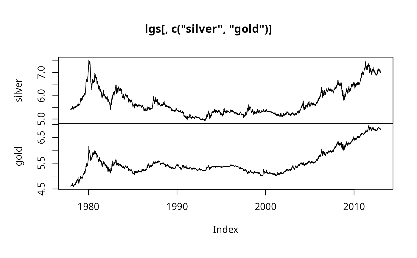
## p.31, daily returns
lgs <- log(GoldSilver)
plot(lgs[, c("silver", "gold")])
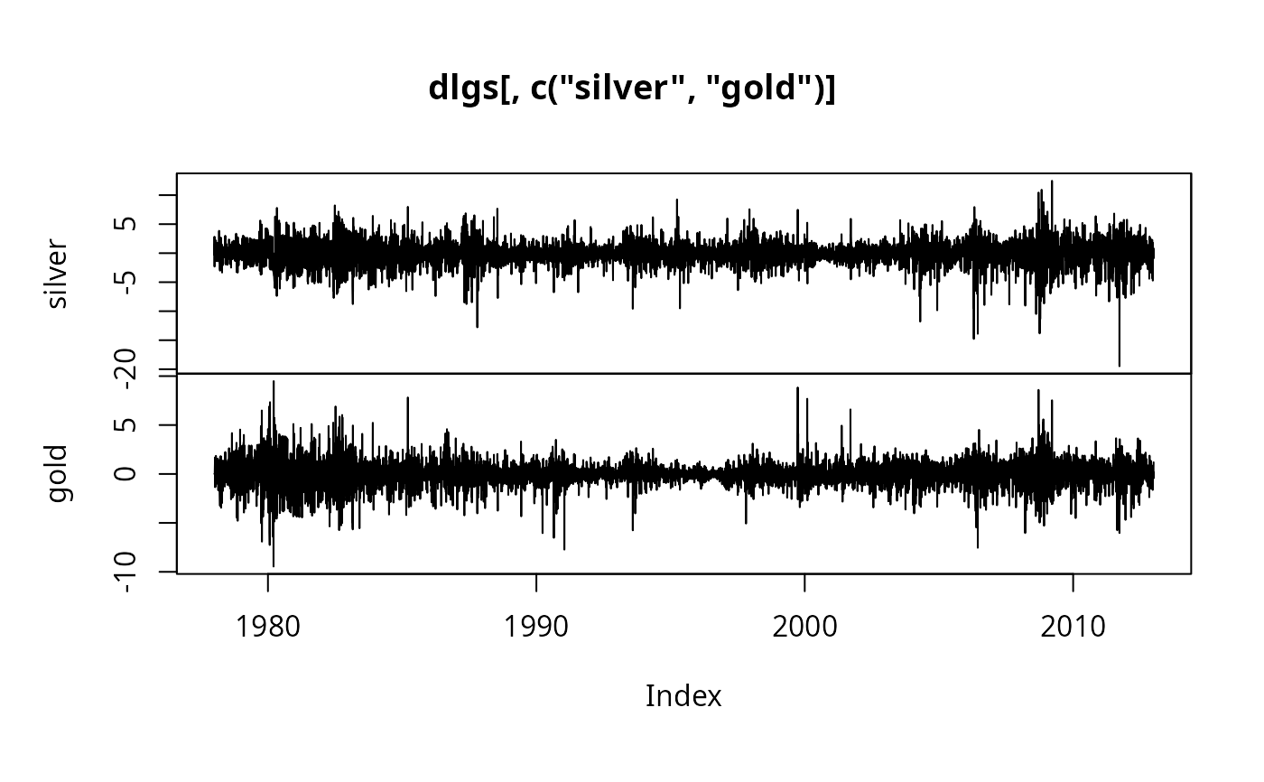
 dlgs <- 100 * diff(lgs)
plot(dlgs[, c("silver", "gold")])
dlgs <- 100 * diff(lgs)
plot(dlgs[, c("silver", "gold")])
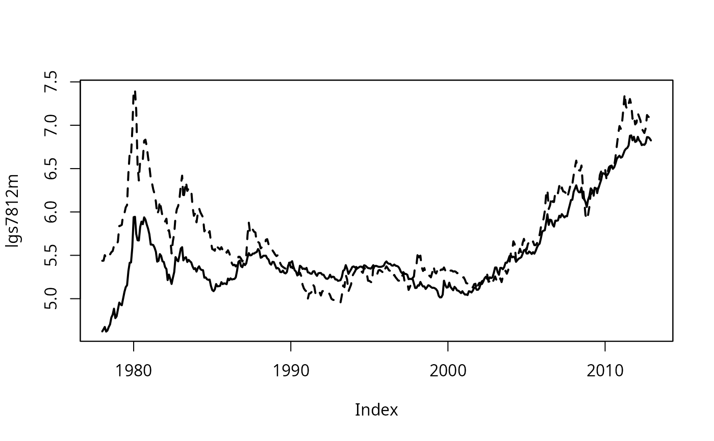
 ## p.31, monthly log prices
lgs7812 <- window(lgs, start = as.Date("1978-01-01"))
lgs7812m <- aggregate(lgs7812, as.Date(as.yearmon(time(lgs7812))), mean)
plot(lgs7812m, plot.type = "single", lty = 1:2, lwd = 2)
## p.31, monthly log prices
lgs7812 <- window(lgs, start = as.Date("1978-01-01"))
lgs7812m <- aggregate(lgs7812, as.Date(as.yearmon(time(lgs7812))), mean)
plot(lgs7812m, plot.type = "single", lty = 1:2, lwd = 2)
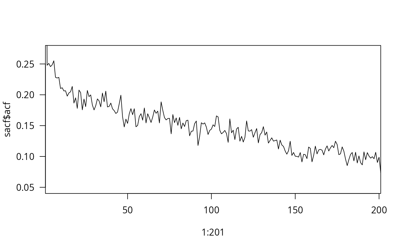
 ## p.93, empirical ACF of absolute daily gold returns, 1978-01-01 - 2012-12-31
absgret <- abs(100 * diff(lgs7812[, "gold"]))
sacf <- acf(absgret, lag.max = 200, na.action = na.exclude, plot = FALSE)
plot(1:201, sacf$acf, ylim = c(0.04, 0.28), type = "l", xaxs = "i", yaxs = "i", las = 1)
## p.93, empirical ACF of absolute daily gold returns, 1978-01-01 - 2012-12-31
absgret <- abs(100 * diff(lgs7812[, "gold"]))
sacf <- acf(absgret, lag.max = 200, na.action = na.exclude, plot = FALSE)
plot(1:201, sacf$acf, ylim = c(0.04, 0.28), type = "l", xaxs = "i", yaxs = "i", las = 1)
 # \donttest{
## ARFIMA(0,1,1) model, eq. (4.44)
library("longmemo")
WhittleEst(absgret, model = "fARIMA", p = 0, q = 1, start = list(H = 0.3, MA = .25))
#> 'WhittleEst' Whittle estimator for fractional ARIMA ('fARIMA'); call:
#> WhittleEst(x = absgret, model = "fARIMA", p = 0, q = 1, start = list(H = 0.3,
#> MA = 0.25))
#> ARMA order (p=0, q=1); time series of length n = 9130.
#>
#> H = 0.8221219
#> coefficients 'eta' =
#> Estimate Std. Error z value Pr(>|z|)
#> H 0.82212189 0.01703983 48.24707 < 2.22e-16
#> MA -0.26559749 0.02096396 -12.66924 < 2.22e-16
#> <==> d := H - 1/2 = 0.322 (0.017)
#>
#> $ vcov : num [1:2, 1:2] 0.00029 -0.000313 -0.000313 0.000439
#> ..- attr(*, "dimnames")=List of 2
#> .. ..$ : chr [1:2] "H" "MA"
#> .. ..$ : chr [1:2] "H" "MA"
#> $ periodogr.x:‘zoo’ series from 1978-01-04 to 1995-07-03
#> Data: num [1:4564] 52.12 4.29 4.45 9.9 4.59 ...
#> Index: Date[1:4564], format: "1978-01-04" "1978-01-05" ...
#> $ spec : num [1:4564, 1] 6.3 4.03 3.1 2.58 2.23 ...
library("forecast")
arfima(as.vector(absgret), max.p = 0, max.q = 1)
#>
#> Call:
#> arfima(y = as.vector(absgret), max.p = 0, max.q = 1)
#>
#> Coefficients:
#> d ma.ma1
#> 0.3492222 0.2972577
#> sigma[eps] = 0.8218654
#> a list with components:
#> [1] "log.likelihood" "n" "msg" "d"
#> [5] "ar" "ma" "covariance.dpq" "fnormMin"
#> [9] "sigma" "stderror.dpq" "correlation.dpq" "h"
#> [13] "d.tol" "M" "hessian.dpq" "length.w"
#> [17] "residuals" "fitted" "call" "x"
#> [21] "series"
# }
## p.254: VAR(2), monthly data for 1986.1 - 2012.12
library("vars")
#> Loading required package: urca
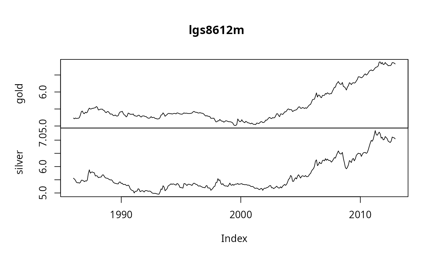
lgs8612 <- window(lgs, start = as.Date("1986-01-01"))
dim(lgs8612)
#> [1] 7044 2
lgs8612m <- aggregate(lgs8612, as.Date(as.yearmon(time(lgs8612))), mean)
plot(lgs8612m)
# \donttest{
## ARFIMA(0,1,1) model, eq. (4.44)
library("longmemo")
WhittleEst(absgret, model = "fARIMA", p = 0, q = 1, start = list(H = 0.3, MA = .25))
#> 'WhittleEst' Whittle estimator for fractional ARIMA ('fARIMA'); call:
#> WhittleEst(x = absgret, model = "fARIMA", p = 0, q = 1, start = list(H = 0.3,
#> MA = 0.25))
#> ARMA order (p=0, q=1); time series of length n = 9130.
#>
#> H = 0.8221219
#> coefficients 'eta' =
#> Estimate Std. Error z value Pr(>|z|)
#> H 0.82212189 0.01703983 48.24707 < 2.22e-16
#> MA -0.26559749 0.02096396 -12.66924 < 2.22e-16
#> <==> d := H - 1/2 = 0.322 (0.017)
#>
#> $ vcov : num [1:2, 1:2] 0.00029 -0.000313 -0.000313 0.000439
#> ..- attr(*, "dimnames")=List of 2
#> .. ..$ : chr [1:2] "H" "MA"
#> .. ..$ : chr [1:2] "H" "MA"
#> $ periodogr.x:‘zoo’ series from 1978-01-04 to 1995-07-03
#> Data: num [1:4564] 52.12 4.29 4.45 9.9 4.59 ...
#> Index: Date[1:4564], format: "1978-01-04" "1978-01-05" ...
#> $ spec : num [1:4564, 1] 6.3 4.03 3.1 2.58 2.23 ...
library("forecast")
arfima(as.vector(absgret), max.p = 0, max.q = 1)
#>
#> Call:
#> arfima(y = as.vector(absgret), max.p = 0, max.q = 1)
#>
#> Coefficients:
#> d ma.ma1
#> 0.3492222 0.2972577
#> sigma[eps] = 0.8218654
#> a list with components:
#> [1] "log.likelihood" "n" "msg" "d"
#> [5] "ar" "ma" "covariance.dpq" "fnormMin"
#> [9] "sigma" "stderror.dpq" "correlation.dpq" "h"
#> [13] "d.tol" "M" "hessian.dpq" "length.w"
#> [17] "residuals" "fitted" "call" "x"
#> [21] "series"
# }
## p.254: VAR(2), monthly data for 1986.1 - 2012.12
library("vars")
#> Loading required package: urca
lgs8612 <- window(lgs, start = as.Date("1986-01-01"))
dim(lgs8612)
#> [1] 7044 2
lgs8612m <- aggregate(lgs8612, as.Date(as.yearmon(time(lgs8612))), mean)
plot(lgs8612m)
 dim(lgs8612m)
#> [1] 324 2
VARselect(lgs8612m, 5)
#> $selection
#> AIC(n) HQ(n) SC(n) FPE(n)
#> 3 2 2 3
#>
#> $criteria
#> 1 2 3 4 5
#> AIC(n) -1.274002e+01 -1.279067e+01 -1.279473e+01 -1.278206e+01 -1.276537e+01
#> HQ(n) -1.271174e+01 -1.274353e+01 -1.272874e+01 -1.269721e+01 -1.266167e+01
#> SC(n) -1.266920e+01 -1.267264e+01 -1.262949e+01 -1.256960e+01 -1.250570e+01
#> FPE(n) 2.931433e-06 2.786669e-06 2.775388e-06 2.810831e-06 2.858202e-06
#>
gs2 <- VAR(lgs8612m, 2)
summary(gs2)
#>
#> VAR Estimation Results:
#> =========================
#> Endogenous variables: gold, silver
#> Deterministic variables: const
#> Sample size: 322
#> Log Likelihood: 1157.62
#> Roots of the characteristic polynomial:
#> 1.006 0.9157 0.249 0.1188
#> Call:
#> VAR(y = lgs8612m, p = 2)
#>
#>
#> Estimation results for equation gold:
#> =====================================
#> gold = gold.l1 + silver.l1 + gold.l2 + silver.l2 + const
#>
#> Estimate Std. Error t value Pr(>|t|)
#> gold.l1 1.06084 0.07385 14.364 <2e-16 ***
#> silver.l1 0.03858 0.04120 0.936 0.350
#> gold.l2 -0.06034 0.07376 -0.818 0.414
#> silver.l2 -0.03454 0.04095 -0.844 0.400
#> const -0.02096 0.02385 -0.879 0.380
#> ---
#> Signif. codes: 0 ‘***’ 0.001 ‘**’ 0.01 ‘*’ 0.05 ‘.’ 0.1 ‘ ’ 1
#>
#>
#> Residual standard error: 0.03519 on 317 degrees of freedom
#> Multiple R-Squared: 0.9952, Adjusted R-squared: 0.9951
#> F-statistic: 1.644e+04 on 4 and 317 DF, p-value: < 2.2e-16
#>
#>
#> Estimation results for equation silver:
#> =======================================
#> silver = gold.l1 + silver.l1 + gold.l2 + silver.l2 + const
#>
#> Estimate Std. Error t value Pr(>|t|)
#> gold.l1 -0.21844 0.12996 -1.681 0.0938 .
#> silver.l1 1.22837 0.07250 16.942 < 2e-16 ***
#> gold.l2 0.29021 0.12980 2.236 0.0261 *
#> silver.l2 -0.28535 0.07206 -3.960 9.26e-05 ***
#> const -0.07413 0.04198 -1.766 0.0784 .
#> ---
#> Signif. codes: 0 ‘***’ 0.001 ‘**’ 0.01 ‘*’ 0.05 ‘.’ 0.1 ‘ ’ 1
#>
#>
#> Residual standard error: 0.06192 on 317 degrees of freedom
#> Multiple R-Squared: 0.9893, Adjusted R-squared: 0.9892
#> F-statistic: 7343 on 4 and 317 DF, p-value: < 2.2e-16
#>
#>
#>
#> Covariance matrix of residuals:
#> gold silver
#> gold 0.001238 0.001442
#> silver 0.001442 0.003834
#>
#> Correlation matrix of residuals:
#> gold silver
#> gold 1.000 0.662
#> silver 0.662 1.000
#>
#>
summary(gs2)$covres
#> gold silver
#> gold 0.001238045 0.001442211
#> silver 0.001442211 0.003834060
## ACF of residuals, p.256
acf(resid(gs2), 2, plot = FALSE)
#>
#> Autocorrelations of series ‘resid(gs2)’, by lag
#>
#> , , gold
#>
#> gold silver
#> 1.000 ( 0) 0.662 ( 0)
#> 0.015 ( 1) 0.012 (-1)
#> -0.138 ( 2) -0.099 (-2)
#>
#> , , silver
#>
#> gold silver
#> 0.662 ( 0) 1.000 ( 0)
#> 0.005 ( 1) 0.018 ( 1)
#> -0.088 ( 2) -0.120 ( 2)
#>
# \donttest{
## Figure 9.1, p.260 (somewhat different)
plot(irf(gs2, impulse = "gold", n.ahead = 50), ylim = c(-0.02, 0.1))
dim(lgs8612m)
#> [1] 324 2
VARselect(lgs8612m, 5)
#> $selection
#> AIC(n) HQ(n) SC(n) FPE(n)
#> 3 2 2 3
#>
#> $criteria
#> 1 2 3 4 5
#> AIC(n) -1.274002e+01 -1.279067e+01 -1.279473e+01 -1.278206e+01 -1.276537e+01
#> HQ(n) -1.271174e+01 -1.274353e+01 -1.272874e+01 -1.269721e+01 -1.266167e+01
#> SC(n) -1.266920e+01 -1.267264e+01 -1.262949e+01 -1.256960e+01 -1.250570e+01
#> FPE(n) 2.931433e-06 2.786669e-06 2.775388e-06 2.810831e-06 2.858202e-06
#>
gs2 <- VAR(lgs8612m, 2)
summary(gs2)
#>
#> VAR Estimation Results:
#> =========================
#> Endogenous variables: gold, silver
#> Deterministic variables: const
#> Sample size: 322
#> Log Likelihood: 1157.62
#> Roots of the characteristic polynomial:
#> 1.006 0.9157 0.249 0.1188
#> Call:
#> VAR(y = lgs8612m, p = 2)
#>
#>
#> Estimation results for equation gold:
#> =====================================
#> gold = gold.l1 + silver.l1 + gold.l2 + silver.l2 + const
#>
#> Estimate Std. Error t value Pr(>|t|)
#> gold.l1 1.06084 0.07385 14.364 <2e-16 ***
#> silver.l1 0.03858 0.04120 0.936 0.350
#> gold.l2 -0.06034 0.07376 -0.818 0.414
#> silver.l2 -0.03454 0.04095 -0.844 0.400
#> const -0.02096 0.02385 -0.879 0.380
#> ---
#> Signif. codes: 0 ‘***’ 0.001 ‘**’ 0.01 ‘*’ 0.05 ‘.’ 0.1 ‘ ’ 1
#>
#>
#> Residual standard error: 0.03519 on 317 degrees of freedom
#> Multiple R-Squared: 0.9952, Adjusted R-squared: 0.9951
#> F-statistic: 1.644e+04 on 4 and 317 DF, p-value: < 2.2e-16
#>
#>
#> Estimation results for equation silver:
#> =======================================
#> silver = gold.l1 + silver.l1 + gold.l2 + silver.l2 + const
#>
#> Estimate Std. Error t value Pr(>|t|)
#> gold.l1 -0.21844 0.12996 -1.681 0.0938 .
#> silver.l1 1.22837 0.07250 16.942 < 2e-16 ***
#> gold.l2 0.29021 0.12980 2.236 0.0261 *
#> silver.l2 -0.28535 0.07206 -3.960 9.26e-05 ***
#> const -0.07413 0.04198 -1.766 0.0784 .
#> ---
#> Signif. codes: 0 ‘***’ 0.001 ‘**’ 0.01 ‘*’ 0.05 ‘.’ 0.1 ‘ ’ 1
#>
#>
#> Residual standard error: 0.06192 on 317 degrees of freedom
#> Multiple R-Squared: 0.9893, Adjusted R-squared: 0.9892
#> F-statistic: 7343 on 4 and 317 DF, p-value: < 2.2e-16
#>
#>
#>
#> Covariance matrix of residuals:
#> gold silver
#> gold 0.001238 0.001442
#> silver 0.001442 0.003834
#>
#> Correlation matrix of residuals:
#> gold silver
#> gold 1.000 0.662
#> silver 0.662 1.000
#>
#>
summary(gs2)$covres
#> gold silver
#> gold 0.001238045 0.001442211
#> silver 0.001442211 0.003834060
## ACF of residuals, p.256
acf(resid(gs2), 2, plot = FALSE)
#>
#> Autocorrelations of series ‘resid(gs2)’, by lag
#>
#> , , gold
#>
#> gold silver
#> 1.000 ( 0) 0.662 ( 0)
#> 0.015 ( 1) 0.012 (-1)
#> -0.138 ( 2) -0.099 (-2)
#>
#> , , silver
#>
#> gold silver
#> 0.662 ( 0) 1.000 ( 0)
#> 0.005 ( 1) 0.018 ( 1)
#> -0.088 ( 2) -0.120 ( 2)
#>
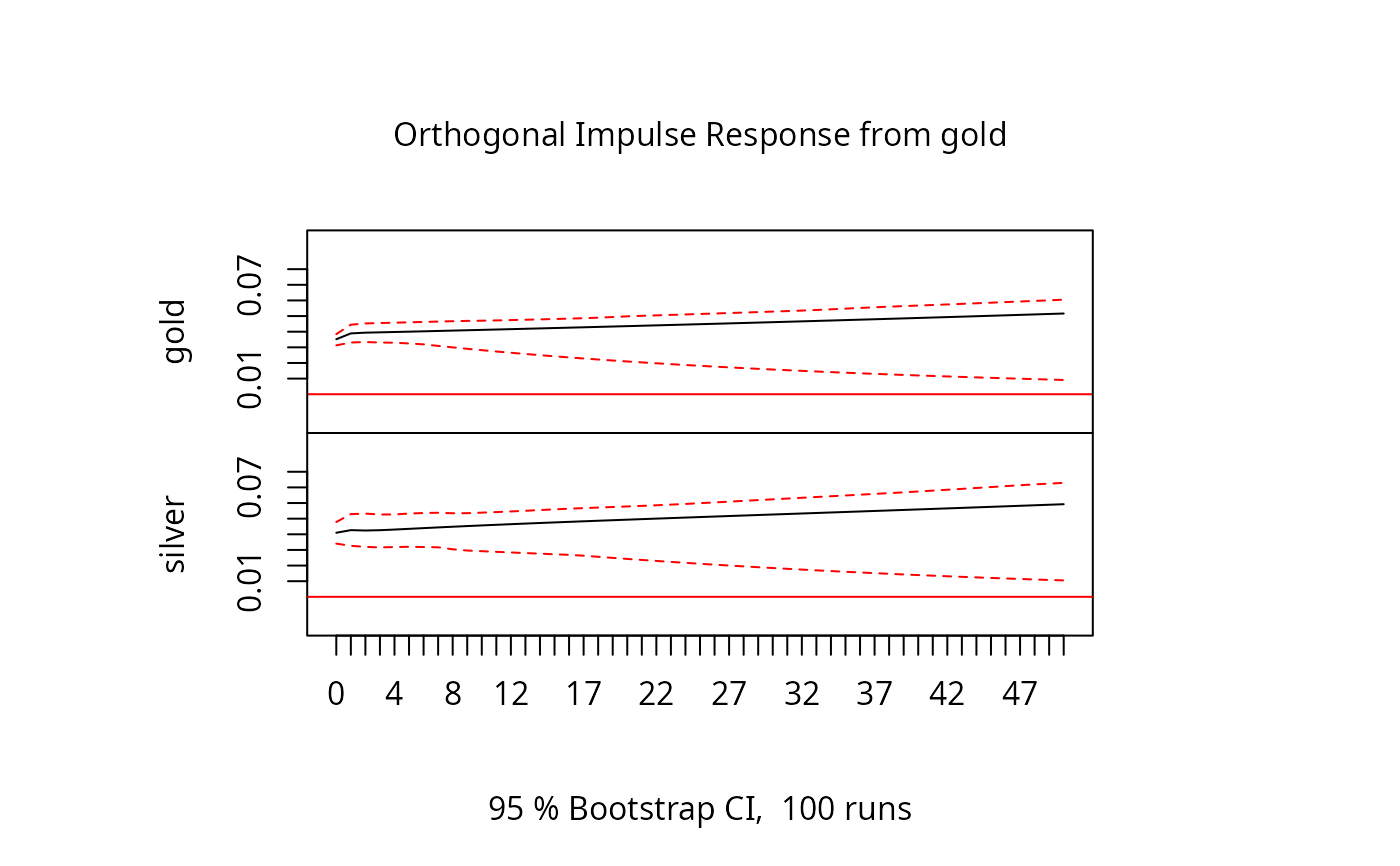
# \donttest{
## Figure 9.1, p.260 (somewhat different)
plot(irf(gs2, impulse = "gold", n.ahead = 50), ylim = c(-0.02, 0.1))
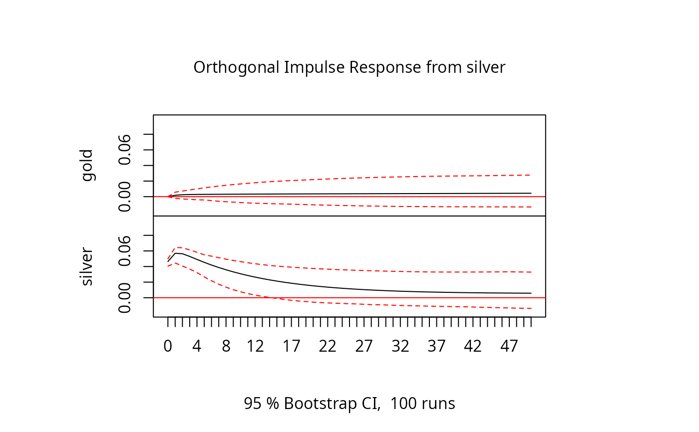
 plot(irf(gs2, impulse = "silver", n.ahead = 50), ylim = c(-0.02, 0.1))
 # }
## Table 9.2, p.261
fevd(gs2)
#> $gold
#> gold silver
#> [1,] 1.0000000 0.000000000
#> [2,] 0.9988365 0.001163524
#> [3,] 0.9978125 0.002187521
#> [4,] 0.9971173 0.002882671
#> [5,] 0.9966392 0.003360835
#> [6,] 0.9962898 0.003710162
#> [7,] 0.9960192 0.003980766
#> [8,] 0.9957996 0.004200378
#> [9,] 0.9956151 0.004384942
#> [10,] 0.9954559 0.004544131
#>
#> $silver
#> gold silver
#> [1,] 0.4381897 0.5618103
#> [2,] 0.3930838 0.6069162
#> [3,] 0.3817063 0.6182937
#> [4,] 0.3845103 0.6154897
#> [5,] 0.3938363 0.6061637
#> [6,] 0.4063921 0.5936079
#> [7,] 0.4206183 0.5793817
#> [8,] 0.4357010 0.5642990
#> [9,] 0.4511753 0.5488247
#> [10,] 0.4667546 0.5332454
#>
## p.266
ls <- lgs8612[, "silver"]
lg <- lgs8612[, "gold"]
gsreg <- lm(lg ~ ls)
summary(gsreg)
#>
#> Call:
#> lm(formula = lg ~ ls)
#>
#> Residuals:
#> Min 1Q Median 3Q Max
#> -0.40097 -0.10317 -0.00179 0.10857 0.33631
#>
#> Coefficients:
#> Estimate Std. Error t value Pr(>|t|)
#> (Intercept) 0.971967 0.015506 62.68 <2e-16 ***
#> ls 0.816752 0.002732 298.92 <2e-16 ***
#> ---
#> Signif. codes: 0 ‘***’ 0.001 ‘**’ 0.01 ‘*’ 0.05 ‘.’ 0.1 ‘ ’ 1
#>
#> Residual standard error: 0.1362 on 7042 degrees of freedom
#> Multiple R-squared: 0.9269, Adjusted R-squared: 0.9269
#> F-statistic: 8.935e+04 on 1 and 7042 DF, p-value: < 2.2e-16
#>
sgreg <- lm(ls ~ lg)
summary(sgreg)
#>
#> Call:
#> lm(formula = ls ~ lg)
#>
#> Residuals:
#> Min 1Q Median 3Q Max
#> -0.3619 -0.1284 0.0074 0.1256 0.5188
#>
#> Coefficients:
#> Estimate Std. Error t value Pr(>|t|)
#> (Intercept) -0.690802 0.021278 -32.47 <2e-16 ***
#> lg 1.134917 0.003797 298.92 <2e-16 ***
#> ---
#> Signif. codes: 0 ‘***’ 0.001 ‘**’ 0.01 ‘*’ 0.05 ‘.’ 0.1 ‘ ’ 1
#>
#> Residual standard error: 0.1605 on 7042 degrees of freedom
#> Multiple R-squared: 0.9269, Adjusted R-squared: 0.9269
#> F-statistic: 8.935e+04 on 1 and 7042 DF, p-value: < 2.2e-16
#>
library("tseries")
adf.test(resid(gsreg), k = 0)
#>
#> Augmented Dickey-Fuller Test
#>
#> data: resid(gsreg)
#> Dickey-Fuller = -3.4284, Lag order = 0, p-value = 0.04912
#> alternative hypothesis: stationary
#>
adf.test(resid(sgreg), k = 0)
#>
#> Augmented Dickey-Fuller Test
#>
#> data: resid(sgreg)
#> Dickey-Fuller = -3.6544, Lag order = 0, p-value = 0.02734
#> alternative hypothesis: stationary
#>
# }
## Table 9.2, p.261
fevd(gs2)
#> $gold
#> gold silver
#> [1,] 1.0000000 0.000000000
#> [2,] 0.9988365 0.001163524
#> [3,] 0.9978125 0.002187521
#> [4,] 0.9971173 0.002882671
#> [5,] 0.9966392 0.003360835
#> [6,] 0.9962898 0.003710162
#> [7,] 0.9960192 0.003980766
#> [8,] 0.9957996 0.004200378
#> [9,] 0.9956151 0.004384942
#> [10,] 0.9954559 0.004544131
#>
#> $silver
#> gold silver
#> [1,] 0.4381897 0.5618103
#> [2,] 0.3930838 0.6069162
#> [3,] 0.3817063 0.6182937
#> [4,] 0.3845103 0.6154897
#> [5,] 0.3938363 0.6061637
#> [6,] 0.4063921 0.5936079
#> [7,] 0.4206183 0.5793817
#> [8,] 0.4357010 0.5642990
#> [9,] 0.4511753 0.5488247
#> [10,] 0.4667546 0.5332454
#>
## p.266
ls <- lgs8612[, "silver"]
lg <- lgs8612[, "gold"]
gsreg <- lm(lg ~ ls)
summary(gsreg)
#>
#> Call:
#> lm(formula = lg ~ ls)
#>
#> Residuals:
#> Min 1Q Median 3Q Max
#> -0.40097 -0.10317 -0.00179 0.10857 0.33631
#>
#> Coefficients:
#> Estimate Std. Error t value Pr(>|t|)
#> (Intercept) 0.971967 0.015506 62.68 <2e-16 ***
#> ls 0.816752 0.002732 298.92 <2e-16 ***
#> ---
#> Signif. codes: 0 ‘***’ 0.001 ‘**’ 0.01 ‘*’ 0.05 ‘.’ 0.1 ‘ ’ 1
#>
#> Residual standard error: 0.1362 on 7042 degrees of freedom
#> Multiple R-squared: 0.9269, Adjusted R-squared: 0.9269
#> F-statistic: 8.935e+04 on 1 and 7042 DF, p-value: < 2.2e-16
#>
sgreg <- lm(ls ~ lg)
summary(sgreg)
#>
#> Call:
#> lm(formula = ls ~ lg)
#>
#> Residuals:
#> Min 1Q Median 3Q Max
#> -0.3619 -0.1284 0.0074 0.1256 0.5188
#>
#> Coefficients:
#> Estimate Std. Error t value Pr(>|t|)
#> (Intercept) -0.690802 0.021278 -32.47 <2e-16 ***
#> lg 1.134917 0.003797 298.92 <2e-16 ***
#> ---
#> Signif. codes: 0 ‘***’ 0.001 ‘**’ 0.01 ‘*’ 0.05 ‘.’ 0.1 ‘ ’ 1
#>
#> Residual standard error: 0.1605 on 7042 degrees of freedom
#> Multiple R-squared: 0.9269, Adjusted R-squared: 0.9269
#> F-statistic: 8.935e+04 on 1 and 7042 DF, p-value: < 2.2e-16
#>
library("tseries")
adf.test(resid(gsreg), k = 0)
#>
#> Augmented Dickey-Fuller Test
#>
#> data: resid(gsreg)
#> Dickey-Fuller = -3.4284, Lag order = 0, p-value = 0.04912
#> alternative hypothesis: stationary
#>
adf.test(resid(sgreg), k = 0)
#>
#> Augmented Dickey-Fuller Test
#>
#> data: resid(sgreg)
#> Dickey-Fuller = -3.6544, Lag order = 0, p-value = 0.02734
#> alternative hypothesis: stationary
#>