Bank Wages
BankWages.RdWages of employees of a US bank.
Usage
data("BankWages")Format
A data frame containing 474 observations on 4 variables.
- job
Ordered factor indicating job category, with levels
"custodial","admin"and"manage".- education
Education in years.
- gender
Factor indicating gender.
- minority
Factor. Is the employee member of a minority?
Source
Online complements to Heij, de Boer, Franses, Kloek, and van Dijk (2004).
https://global.oup.com/booksites/content/0199268010/datasets/ch6/xr614bwa.asc
References
Heij, C., de Boer, P.M.C., Franses, P.H., Kloek, T. and van Dijk, H.K. (2004). Econometric Methods with Applications in Business and Economics. Oxford: Oxford University Press.
Examples
#> Loading required namespace: nnet
#> Loading required namespace: mlogit
data("BankWages")
## exploratory analysis of job ~ education
## (tables and spine plots, some education levels merged)
xtabs(~ education + job, data = BankWages)
#> job
#> education custodial admin manage
#> 8 13 40 0
#> 12 13 176 1
#> 14 0 6 0
#> 15 1 111 4
#> 16 0 24 35
#> 17 0 3 8
#> 18 0 2 7
#> 19 0 1 26
#> 20 0 0 2
#> 21 0 0 1
edcat <- factor(BankWages$education)
levels(edcat)[3:10] <- rep(c("14-15", "16-18", "19-21"), c(2, 3, 3))
tab <- xtabs(~ edcat + job, data = BankWages)
prop.table(tab, 1)
#> job
#> edcat custodial admin manage
#> 8 0.245283019 0.754716981 0.000000000
#> 12 0.068421053 0.926315789 0.005263158
#> 14-15 0.008196721 0.959016393 0.032786885
#> 16-18 0.000000000 0.367088608 0.632911392
#> 19-21 0.000000000 0.033333333 0.966666667
spineplot(tab, off = 0)
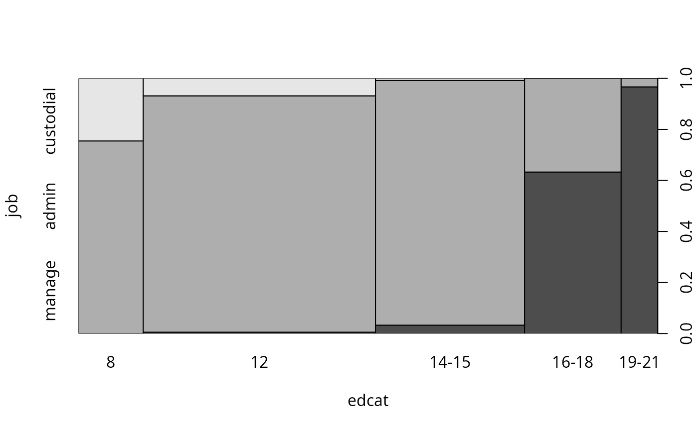 plot(job ~ edcat, data = BankWages, off = 0)
## fit multinomial model for male employees
library("nnet")
fm_mnl <- multinom(job ~ education + minority, data = BankWages,
subset = gender == "male", trace = FALSE)
summary(fm_mnl)
#> Call:
#> multinom(formula = job ~ education + minority, data = BankWages,
#> subset = gender == "male", trace = FALSE)
#>
#> Coefficients:
#> (Intercept) education minorityyes
#> admin -4.760725 0.5533995 -0.4269495
#> manage -30.774855 2.1867717 -2.5360409
#>
#> Std. Errors:
#> (Intercept) education minorityyes
#> admin 1.172774 0.09904108 0.5027084
#> manage 4.478612 0.29483562 0.9342070
#>
#> Residual Deviance: 237.472
#> AIC: 249.472
confint(fm_mnl)
#> , , admin
#>
#> 2.5 % 97.5 %
#> (Intercept) -7.0593203 -2.4621301
#> education 0.3592825 0.7475164
#> minorityyes -1.4122398 0.5583409
#>
#> , , manage
#>
#> 2.5 % 97.5 %
#> (Intercept) -39.552774 -21.9969368
#> education 1.608904 2.7646389
#> minorityyes -4.367053 -0.7050288
#>
## same with mlogit package
library("mlogit")
#> Loading required package: dfidx
#>
#> Attaching package: ‘mlogit’
#> The following object is masked from ‘package:plm’:
#>
#> has.intercept
fm_mlogit <- mlogit(job ~ 1 | education + minority, data = BankWages,
subset = gender == "male", shape = "wide", reflevel = "custodial")
summary(fm_mlogit)
#>
#> Call:
#> mlogit(formula = job ~ 1 | education + minority, data = BankWages,
#> subset = gender == "male", reflevel = "custodial", shape = "wide",
#> method = "nr")
#>
#> Frequencies of alternatives:choice
#> custodial admin manage
#> 0.10465 0.60853 0.28682
#>
#> nr method
#> 8 iterations, 0h:0m:0s
#> g'(-H)^-1g = 9.15E-06
#> successive function values within tolerance limits
#>
#> Coefficients :
#> Estimate Std. Error z-value Pr(>|z|)
#> (Intercept):admin -4.760722 1.172774 -4.0594 4.921e-05 ***
#> (Intercept):manage -30.774826 4.478608 -6.8715 6.352e-12 ***
#> education:admin 0.553399 0.099041 5.5876 2.303e-08 ***
#> education:manage 2.186770 0.294835 7.4169 1.199e-13 ***
#> minorityyes:admin -0.426952 0.502708 -0.8493 0.395712
#> minorityyes:manage -2.536041 0.934207 -2.7146 0.006635 **
#> ---
#> Signif. codes: 0 ‘***’ 0.001 ‘**’ 0.01 ‘*’ 0.05 ‘.’ 0.1 ‘ ’ 1
#>
#> Log-Likelihood: -118.74
#> McFadden R^2: 0.48676
#> Likelihood ratio test : chisq = 225.22 (p.value = < 2.22e-16)
plot(job ~ edcat, data = BankWages, off = 0)
## fit multinomial model for male employees
library("nnet")
fm_mnl <- multinom(job ~ education + minority, data = BankWages,
subset = gender == "male", trace = FALSE)
summary(fm_mnl)
#> Call:
#> multinom(formula = job ~ education + minority, data = BankWages,
#> subset = gender == "male", trace = FALSE)
#>
#> Coefficients:
#> (Intercept) education minorityyes
#> admin -4.760725 0.5533995 -0.4269495
#> manage -30.774855 2.1867717 -2.5360409
#>
#> Std. Errors:
#> (Intercept) education minorityyes
#> admin 1.172774 0.09904108 0.5027084
#> manage 4.478612 0.29483562 0.9342070
#>
#> Residual Deviance: 237.472
#> AIC: 249.472
confint(fm_mnl)
#> , , admin
#>
#> 2.5 % 97.5 %
#> (Intercept) -7.0593203 -2.4621301
#> education 0.3592825 0.7475164
#> minorityyes -1.4122398 0.5583409
#>
#> , , manage
#>
#> 2.5 % 97.5 %
#> (Intercept) -39.552774 -21.9969368
#> education 1.608904 2.7646389
#> minorityyes -4.367053 -0.7050288
#>
## same with mlogit package
library("mlogit")
#> Loading required package: dfidx
#>
#> Attaching package: ‘mlogit’
#> The following object is masked from ‘package:plm’:
#>
#> has.intercept
fm_mlogit <- mlogit(job ~ 1 | education + minority, data = BankWages,
subset = gender == "male", shape = "wide", reflevel = "custodial")
summary(fm_mlogit)
#>
#> Call:
#> mlogit(formula = job ~ 1 | education + minority, data = BankWages,
#> subset = gender == "male", reflevel = "custodial", shape = "wide",
#> method = "nr")
#>
#> Frequencies of alternatives:choice
#> custodial admin manage
#> 0.10465 0.60853 0.28682
#>
#> nr method
#> 8 iterations, 0h:0m:0s
#> g'(-H)^-1g = 9.15E-06
#> successive function values within tolerance limits
#>
#> Coefficients :
#> Estimate Std. Error z-value Pr(>|z|)
#> (Intercept):admin -4.760722 1.172774 -4.0594 4.921e-05 ***
#> (Intercept):manage -30.774826 4.478608 -6.8715 6.352e-12 ***
#> education:admin 0.553399 0.099041 5.5876 2.303e-08 ***
#> education:manage 2.186770 0.294835 7.4169 1.199e-13 ***
#> minorityyes:admin -0.426952 0.502708 -0.8493 0.395712
#> minorityyes:manage -2.536041 0.934207 -2.7146 0.006635 **
#> ---
#> Signif. codes: 0 ‘***’ 0.001 ‘**’ 0.01 ‘*’ 0.05 ‘.’ 0.1 ‘ ’ 1
#>
#> Log-Likelihood: -118.74
#> McFadden R^2: 0.48676
#> Likelihood ratio test : chisq = 225.22 (p.value = < 2.22e-16)